Homework 3 (due March 22nd 9pm)

Stat 154/254: Statistical Machine Learning

1 ROC curves of bad classifiers

(a)

Let \(x\sim \mathcal{N}\left(0, 1\right)\) be drawn independently of \(y\in \{0, 1\}\). Plot the ROC curve for the family of classifiers \(\hat{f}(x| t) = \mathrm{I}\left(x> t\right)\) indexed by \(t\in \mathbb{R}^{}\).

(b)

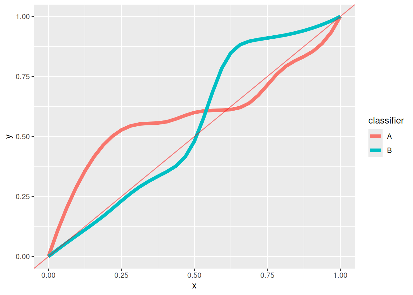
Suppose you have two not–so–great classifiers, A and B, with the following ROC curves. How can you combine them to get a better one?

(c)

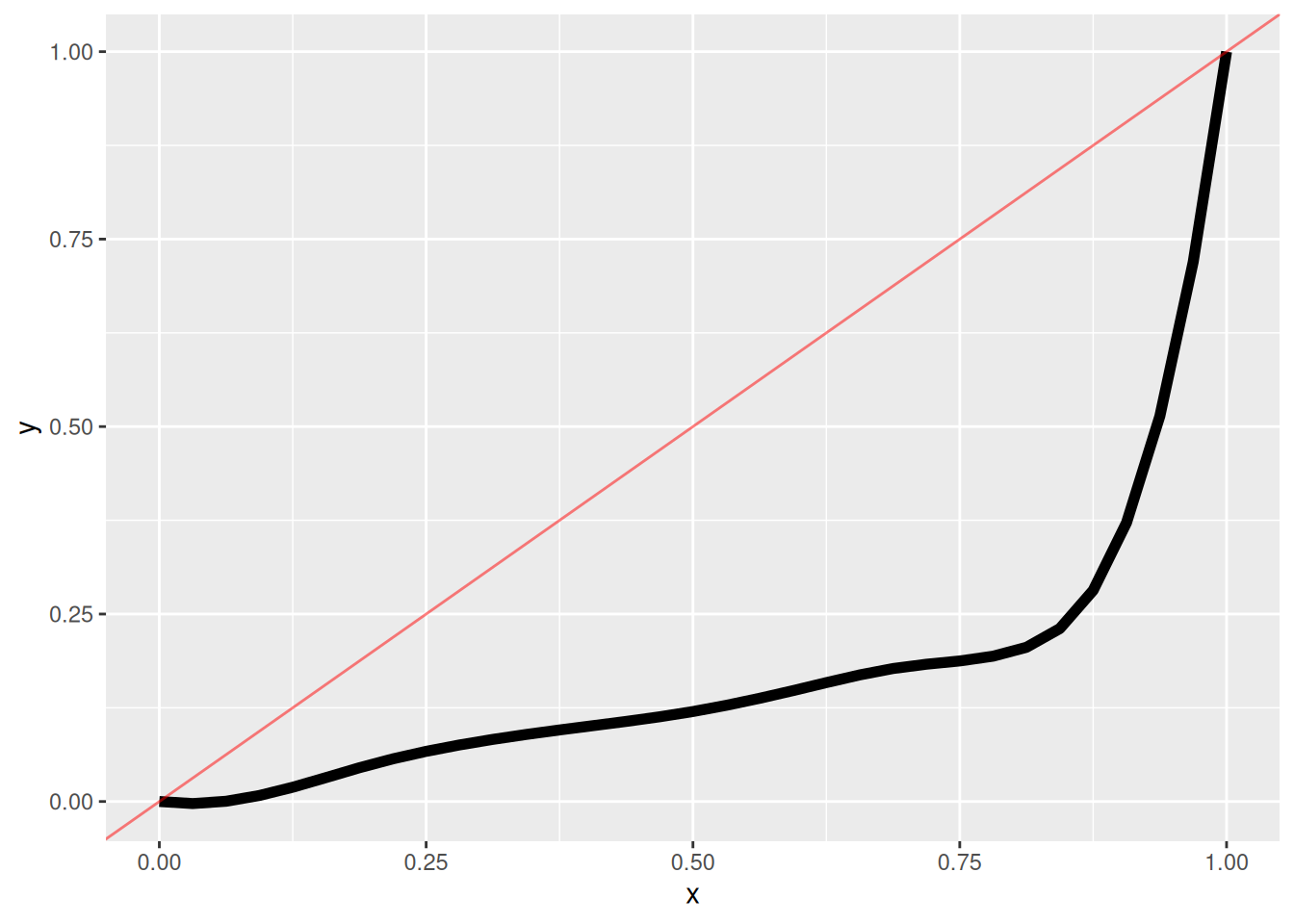
Suppose you have the a terrible classifier with the following ROC curve. How can you use it to make a really good classifier?

Solutions

(a) The plot should be a forty–five degree line — at any \(t\), both the true and false rejection rates will be equal to \(p(x> t)\).

(b) I’ll give two possible answers. Full credit for the homework can be given for either solution or for variants — the main idea is to combine classifiers to get a better one.

One solution is to find the thresholds at which classifier A and classifier B’s ROC curves interesect. Call these thresholds \(t_A\) and \(t_B\), respectively. Then you could make a family of classifiers that use classifer \(A\) with \(t< t_A\) and classifier \(B\) with \(t > t_B\).

A better solution is to use randomized classifiers to form the convex hull of the ROC curves. For any thresholds \(t_A\) and \(t_B\) (possibly distinct from the preceding paragraph), you can classify according to \(A\) with probability \(p\) and \(B\) with probability \(1-p\). The TPR and FPR of the randomized classifier lies a proportion \(p\) along a line between the two points on the ROC curve. You can thus form a feasible classifier that connects any pair of points on the two ROC curves; applied to all points, if follows that there exist randomized classifiers achieving any point in the convex hull of the two ROC curves. An example is shown in purple between the two “humps” of the ROC curves:

Warning in geom_segment(aes(x = 0.25, y = 0.53, xend = 0.645, yend = 0.875), : All aesthetics have length 1, but the data has 66 rows.
ℹ Please consider using `annotate()` or provide this layer with data containing
  a single row.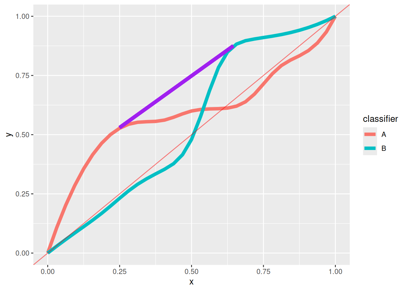

(c)

Just flip the classifier — take \(\hat{y}' = \mathrm{I}\left(\hat{y}= 0\right)\). This produces a classifier that is better than chance, rather than the current classifier, which is worse than chance.

2 The behavior of logistic regression with a separating hyperplane

Consider logistic loss \(\hat{\mathscr{L}}(\boldsymbol{\beta})\) with regressors \(\boldsymbol{x}_n\) and binary responses \(y_n\). Suppose that the data is separable, meaning there exists a \(\boldsymbol{\beta}^{*}\) such that the data is perfectly classified by \(\boldsymbol{\beta}^{*}\):

\[ y_n = 1 \textrm{ if and only if }{\boldsymbol{\beta}^{*}}^\intercal\boldsymbol{x}_n > 0. \]

(a)

Show that the data is also perfectly classified by \(C \boldsymbol{\beta}^{*}\) for any constant \(C > 0\).

(b)

Write an expression for the loss \(\hat{\mathscr{L}}(C \boldsymbol{\beta}^{*})\). What happens to the loss as \(C \rightarrow \infty\)?

(c)

Can there be any solution to the equation \(\partial \hat{\mathscr{L}}(\boldsymbol{\beta}) / \partial \boldsymbol{\beta}= \boldsymbol{0}\)? (Recally that \(\hat{\mathscr{L}}(\boldsymbol{\beta})\) is convex, and so any such solution would be at a global minimum.)

(d)

What will happen if you try to numerically optimize \(\mathscr{L}(\boldsymbol{\beta})\), for example by gradient descent?

Solutions

(a)

\[ {\boldsymbol{\beta}^{*}}^\intercal\boldsymbol{x}_n > 0 \quad\Leftrightarrow\quad C {\boldsymbol{\beta}^{*}}^\intercal\boldsymbol{x}_n > 0 \]

becuase \(C > 0\).

(b)

Let \(\pi^*_n = \exp(C \boldsymbol{x}_n^\intercal\boldsymbol{\beta}^{*}) / (1 + C \boldsymbol{x}_n^\intercal\boldsymbol{\beta}^{*})\). As \(C \rightarrow \infty\), \(\pi^*_n \rightarrow 1\) if \(\boldsymbol{x}_n^\intercal\boldsymbol{\beta}^{*}> 0\) and \(\pi^*_n \rightarrow 0\) if \(\boldsymbol{x}_n^\intercal\boldsymbol{\beta}^{*}< 0\). \[ \begin{aligned} \hat{\mathscr{L}}(C \boldsymbol{\beta}^{*}) ={}& - \frac{1}{N} \sum_{n=1}^N\left(y_n \log \pi^*_n + (1 - y_n) \log(1 - \pi^*_n) \right) \\={}& - \frac{1}{N}\sum_{n:y_n = 1} \log \pi^*_n - \frac{1}{N}\sum_{n:y_n = 0} \log(1 - \pi^*_n) \\={}& - \frac{1}{N}\sum_{n:\boldsymbol{x}_n^\intercal\boldsymbol{\beta}^{*}> 0} \log \pi^*_n - \frac{1}{N}\sum_{n:\boldsymbol{x}_n^\intercal\boldsymbol{\beta}^{*}< 0} \log(1 - \pi^*_n), \end{aligned} \]

where the final line follows from the fact that \(y_n\) is perfectly classified by \(C \boldsymbol{\beta}^{*}\). As a consequence, \(\lim_{C \rightarrow \infty} \hat{\mathscr{L}}(C \boldsymbol{\beta}^{*}) = \log 1 = 0\), but \(\hat{\mathscr{L}}(C \boldsymbol{\beta}^{*}) > 0\) for any finite \(C\).

(c)

By the argument in (b), there cannot be any such point, since the empirical loss decreases without bound in the direction \(C\boldsymbol{\beta}^{*}\).

(d)

If the optimization algorithm is able to find the separating hyperplane, it will continue to make the vector \(\boldsymbol{\beta}\) larger and larger in magnitude until there is some floating point error.

3 Logistic regression as Gaussian generative modeling

In this problem, we will derive a classification technique known as “linear descriminant anlalysis” (LDA). (Not to be confused with “latent Dirichlet allocation,” which is a completely different ML technique for topic modeling.)

Suppose that classification data follows a generative model

\[ p(\boldsymbol{x}\vert y= 0) = \mathcal{N}\left(\boldsymbol{x}| \boldsymbol{\mu}_0, \boldsymbol{\Sigma}\right) \quad\textrm{and}\quad p(\boldsymbol{x}\vert y= 1) = \mathcal{N}\left(\boldsymbol{x}| \boldsymbol{\mu}_1, \boldsymbol{\Sigma}\right) \]

for some covariance matrix \(\boldsymbol{\Sigma}\) and two vectors \(\boldsymbol{\mu}_0\) and \(\boldsymbol{\mu}_1\). Suppose also that \(\mathbb{P}_{\,}\left(y= 1\right) = \mathbb{P}_{\,}\left(y= 0\right) = 0.5\), marginally.

Recall that the multivarite normal density is given by

\[ \mathcal{N}\left(\boldsymbol{x}| \boldsymbol{\mu}, \boldsymbol{\Sigma}\right) = \exp\left( -\frac{1}{2}(\boldsymbol{x}- \boldsymbol{\mu})^\intercal\boldsymbol{\Sigma}^{-1} (\boldsymbol{x}- \boldsymbol{\mu}) - \frac{1}{2} \log |\boldsymbol{\Sigma}| + C \right), \]

where the normalizing constant \(C\) does not depend on \(\boldsymbol{x}\), \(\boldsymbol{\mu}\), or \(\boldsymbol{\Sigma}\). You may assume that \(\boldsymbol{\Sigma}\) is invertible and that the \(\boldsymbol{\mu}_1\) and \(\boldsymbol{\mu}_0\) are distinct.

In this problem, we will compute the optimal classifier in closed form for this setting.

(a)

Show that \[ \frac{\mathbb{P}_{\,}\left(y=1\vert\boldsymbol{x}\right)}{\mathbb{P}_{\,}\left(y=0\vert\boldsymbol{x}\right)} = \frac{\mathbb{P}_{\,}\left(\boldsymbol{x}\vert y=1\right)}{\mathbb{P}_{\,}\left(\boldsymbol{x}\vert y=0\right)}. \] Meaning, the posterior probability ratio equals the likehood ratio, in the case that the priors equal.

Hint: Use Bayes’ formula.

(b)

Express the log likelihood ratio \[ \log \frac{\mathbb{P}_{\,}\left(\boldsymbol{x}\vert y=1\right)}{\mathbb{P}_{\,}\left(\boldsymbol{x}\vert y=0\right)} \]

in terms of \(\boldsymbol{x},\boldsymbol{\mu}_0,\boldsymbol{\mu}_1,\boldsymbol{\Sigma}\), and show that it is affine in \(\boldsymbol{x}\).

(c)

Let \(\hat{f}(\boldsymbol{x})\) be the classifier that predicts the class with the higher posterior probability given \(\boldsymbol{x}\). Use (a) and (b) to show that \[ \hat{f}(\boldsymbol{x}) = 1 \iff \boldsymbol{x}^T\boldsymbol{\beta}^* > c^*, \] where \(\boldsymbol{\beta}^* =\boldsymbol{\Sigma}^{-1}(\boldsymbol{\mu}_1-\boldsymbol{\mu}_0)\), and \(c^*\) is a constant that depends on \(\boldsymbol{\mu}_0,\boldsymbol{\mu}_1,\boldsymbol{\Sigma}\) but not on \(\boldsymbol{x}\). Connect this conclusion to logistic regression.

Solutions

(a)

Using Bayes’ rule twice, \[ \frac{\mathbb{P}_{\,}\left(y=1\vert\boldsymbol{x}\right)}{\mathbb{P}_{\,}\left(y=0\vert\boldsymbol{x}\right)} = \frac{\mathbb{P}_{\,}\left(y=1, \boldsymbol{x}\right) / \mathbb{P}_{\,}\left(\boldsymbol{x}\right)}{\mathbb{P}_{\,}\left(y=0, \boldsymbol{x}\right) / \mathbb{P}_{\,}\left(\boldsymbol{x}\right)} = \frac{\mathbb{P}_{\,}\left(\boldsymbol{x}\vert y=1\right) \mathbb{P}_{\,}\left(y= 1\right) / \mathbb{P}_{\,}\left(\boldsymbol{x}\right)}{\mathbb{P}_{\,}\left(\boldsymbol{x}\vert y= 0\right) \mathbb{P}_{\,}\left(y= 0\right) / \mathbb{P}_{\,}\left(\boldsymbol{x}\right)} = \frac{\mathbb{P}_{\,}\left(\boldsymbol{x}\vert y=1\right)}{\mathbb{P}_{\,}\left(\boldsymbol{x}\vert y= 0\right)}, \]

where the final line uses the fact that \(\mathbb{P}_{\,}\left(y= 1\right) = \mathbb{P}_{\,}\left(y= 0\right) = 1/2\).

(b)

\[ \begin{aligned} \log \frac{\mathbb{P}_{\,}\left(\boldsymbol{x}\vert y=1\right)}{\mathbb{P}_{\,}\left(\boldsymbol{x}\vert y=0\right)} ={}& \log \mathbb{P}_{\,}\left(\boldsymbol{x}\vert y=1\right) - \log \mathbb{P}_{\,}\left(\boldsymbol{x}\vert y=0\right) \\={}& -\frac{1}{2}(\boldsymbol{x}- \boldsymbol{\mu}_1)^\intercal\boldsymbol{\Sigma}^{-1} (\boldsymbol{x}- \boldsymbol{\mu}_1) - \frac{1}{2} \log |\boldsymbol{\Sigma}| + C + \\{}& \frac{1}{2}(\boldsymbol{x}- \boldsymbol{\mu}_0)^\intercal\boldsymbol{\Sigma}^{-1} (\boldsymbol{x}- \boldsymbol{\mu}_0) + \frac{1}{2} \log |\boldsymbol{\Sigma}| - C \\={}& -\frac{1}{2}(\boldsymbol{x}- \boldsymbol{\mu}_1)^\intercal\boldsymbol{\Sigma}^{-1} (\boldsymbol{x}- \boldsymbol{\mu}_1) + \frac{1}{2}(\boldsymbol{x}- \boldsymbol{\mu}_0)^\intercal\boldsymbol{\Sigma}^{-1} (\boldsymbol{x}- \boldsymbol{\mu}_0) \\={}& -\frac{1}{2} \boldsymbol{\mu}_1^\intercal\boldsymbol{\Sigma}^{-1} \boldsymbol{\mu}_1 + \frac{1}{2} \boldsymbol{\mu}_0^\intercal\boldsymbol{\Sigma}^{-1} \boldsymbol{\mu}_0 + \boldsymbol{x}^\intercal\boldsymbol{\Sigma}^{-1} \boldsymbol{\mu}_1 - \boldsymbol{x}^\intercal\boldsymbol{\Sigma}^{-1} \boldsymbol{\mu}_0 \\={}& -\frac{1}{2} \boldsymbol{\mu}_1^\intercal\boldsymbol{\Sigma}^{-1} \boldsymbol{\mu}_1 + \frac{1}{2} \boldsymbol{\mu}_0^\intercal\boldsymbol{\Sigma}^{-1} \boldsymbol{\mu}_0 + \boldsymbol{x}^\intercal\boldsymbol{\Sigma}^{-1} (\boldsymbol{\mu}_1 - \boldsymbol{\mu}_0). \end{aligned} \]

This takes the form \(b+ \boldsymbol{a}^\intercal\boldsymbol{x}\) where \(b= -\frac{1}{2} \boldsymbol{\mu}_1^\intercal\boldsymbol{\Sigma}^{-1} \boldsymbol{\mu}_1 + \frac{1}{2} \boldsymbol{\mu}_0^\intercal\boldsymbol{\Sigma}^{-1} \boldsymbol{\mu}_0\) and \(\boldsymbol{a}= \boldsymbol{\Sigma}^{-1} (\boldsymbol{\mu}_1 - \boldsymbol{\mu}_0)\).

(c)

Combining (a) and (b), we set \(\hat{f}(\boldsymbol{x}) = 1\) when

\[ \begin{aligned} \frac{\mathbb{P}_{\,}\left(y= 1\vert \boldsymbol{x}\right)}{\mathbb{P}_{\,}\left(y=0 \vert \boldsymbol{x}\right)} \ge{}& 1 \quad\Leftrightarrow \\ \frac{\mathbb{P}_{\,}\left(\boldsymbol{x}\vert y=1\right)}{\mathbb{P}_{\,}\left(\boldsymbol{x}\vert y=0\right)} \ge{}& 1 \quad\Leftrightarrow \\ \log \frac{\mathbb{P}_{\,}\left(\boldsymbol{x}\vert y=1\right)}{\mathbb{P}_{\,}\left(\boldsymbol{x}\vert y=0\right)} \ge{}& 0 \quad\Leftrightarrow\\ \boldsymbol{x}^\intercal\boldsymbol{\Sigma}^{-1} (\boldsymbol{\mu}_1 - \boldsymbol{\mu}_0) \ge{}& \frac{1}{2} \boldsymbol{\mu}_1^\intercal\boldsymbol{\Sigma}^{-1} \boldsymbol{\mu}_1 - \frac{1}{2} \boldsymbol{\mu}_0^\intercal\boldsymbol{\Sigma}^{-1} \boldsymbol{\mu}_0. \end{aligned} \]

Logistic regression (with a constant in the regrsesion) also tries to find an affine decision boundary, but does so in a fundamentally different way — by minimizing the cross–entropy loss. Both LDA and logistic regression thus result in affine decision boundaries, but different affine decision boundaries.

4 VC dimension of linear classifiers

Note: this problem uses a definition of VC dimension that is off by one. The size of the shatterable and unshatterable sets are all that matter for full credit.

Consider the class of \(P\)–dimensional linear binary classifiers, \(\mathcal{F}= \{ \mathrm{I}\left(\boldsymbol{x}^\intercal\boldsymbol{\beta}\ge 0\right) \textrm{ for any }\boldsymbol{\beta}\in \mathbb{R}^{P}\}\). In this problem, we will show that the VC dimension of \(\mathcal{F}\) is \(P + 1\), and so proving a generalization bound for logistic regression with zero–one loss.

For \(N\) points, let \(\boldsymbol{X}\) denote the \(N \times P\) matrix with \(\boldsymbol{x}_n^\intercal\) in row \(n\).

First, we show that we can shatter any set of size \(P\) in (a)–(c), showing that the VC dimension is greater than \(P\). Then, in (d)–(f) we show that we cannot shatter a set of size \(P + 1\). Together, this gives that the VC dimension is less than or equal to \(P+1\).

(a)

For any \(y_1, \ldots, y_N\), define \(z_n = 2 y_n - 1\). Show that \(y_n\) is correctly classified if we can find \(\hat{\boldsymbol{\beta}}\) such that \(\hat{\boldsymbol{\beta}}^\intercal\boldsymbol{x}= z_n\).

(b)

When \(N=P\), identify an \(\boldsymbol{X}\) so that, for any \(\boldsymbol{Z}\in \mathbb{R}^{P}\), you can find a \(\hat{\boldsymbol{\beta}}\) such that \(\boldsymbol{X}\hat{\boldsymbol{\beta}}= \boldsymbol{Z}\). Hint: There are actually an infinite number of \(\boldsymbol{X}\) that will work, but also some that won’t.

(c)

Use (a) and the \(\boldsymbol{X}\) you identified in (b) to conclude that you can shatter a set of size \(P\).

(d)

Since \(\boldsymbol{X}'\) is rank \(P\).

Suppose that \(N = P + 1\), and let \(\boldsymbol{X}\) be a matrix of rank \(P\). Let \(\boldsymbol{X}'\) denote the \(P \times P\) matrix containing only the first \(P\) rows of \(\boldsymbol{X}\), and assume that \(\boldsymbol{X}'\) is rank \(P\) without loss of generality. Show that, for any set of \(\boldsymbol{x}_n\), you can find \(\boldsymbol{\gamma}\) such that \(\boldsymbol{x}_{P+1} = \sum_{n=1}^P \gamma_n \boldsymbol{x}_{n}\). That is, show that the final row is a linear combination of the other rows.

(e)

Suppose we have \(y_n = \mathrm{I}\left(\gamma_n > 0\right)\) for \(n=1,\ldots,P\), and suppose that \(\hat{\boldsymbol{\beta}}\) correctly classifies these first \(P\) points. Using (d), show that \(\hat{\boldsymbol{\beta}}^\intercal\boldsymbol{x}_{P+1} \ge 0\).

(f)

Using (e), define a set of \(P+1\) points that cannot be shattered.

(g)

What can you conclude about the generalization error of linear classifiers with zero–one loss? Specifically, what happens to \[ \sup_{f \in \mathcal{F}} \left|\frac{1}{N} \sum_{n=1}^N\mathrm{I}\left(f(\boldsymbol{x}_n) \ne y_n\right) - \mathbb{P}_{\,}\left(f(\boldsymbol{x}) \ne y\right)\right| \]

as \(N \rightarrow \infty\)?

(h)

Let \(\hat{\boldsymbol{\beta}}\) denote the estimate from logistic regression (which was trained with logistic loss, not the zero–one loss), and consider the binary classifier \(f(\boldsymbol{x}; \boldsymbol{\beta}) = \mathrm{I}\left(\boldsymbol{x}^\intercal\boldsymbol{\beta}\ge 0\right)\). What can you conclude about

\[ \left|\frac{1}{N} \sum_{n=1}^N\mathrm{I}\left(f(\boldsymbol{x}; \hat{\boldsymbol{\beta}}) \ne y_n\right) - \mathbb{P}_{\,}\left(f(\boldsymbol{x}; \hat{\boldsymbol{\beta}}) \ne y\right)\right| \]

as \(N \rightarrow \infty\)?

Solutions

(a)

As defined, \(z_n = 1\) when \(y_n = 1\) and \(z_n = -1\) when \(y_n = 0\). So if \(\hat{\boldsymbol{\beta}}^\intercal\boldsymbol{x}= z_n\), then \(\hat{\boldsymbol{\beta}}^\intercal\boldsymbol{x}\) has the correct sign to classify \(y_n\). Of course this is a sufficient, not a necessary condition — it may be that \(y_n\) is correctly classified but \(\hat{\boldsymbol{\beta}}^\intercal\boldsymbol{x}\ne z_n\).

(b)

Any full–rank \(\boldsymbol{X}\) will do, since we can then take \(\hat{\boldsymbol{\beta}}= \boldsymbol{X}^{-1} \boldsymbol{Z}\). This is of course impossible if \(N > P\).

(c)

Take a full–rank \(\boldsymbol{X}\), take any \(\boldsymbol{Y}\in \{0,1\}^P\), take \(\boldsymbol{Z}= 2 \boldsymbol{Y}- 1\), and \(\hat{\boldsymbol{\beta}}= \boldsymbol{X}^{-1}\boldsymbol{Z}\). Then \(\hat{\boldsymbol{\beta}}\) correctly classifies \(\boldsymbol{Y}\). Since this is possible for any of the \(2^P\) possible values of \(\boldsymbol{Y}\), the set given by \(\boldsymbol{X}\) can be shattered.

(d)

Since \(\boldsymbol{X}'\) is rank \(P\), any vector — including \(\boldsymbol{x}_{P+1}\) — can be written as a linear combiantion of the rows of \(\boldsymbol{X}'\).

Note: The problem is a little ambiguous as originally stated. The whole point of this proof is to show that no set of \(P + 1\) points can be shattered, and the only thing that matters is that one regressor is a linear combination of the others. However, that vector need not necessarily be the last row. Give full credit for any variants that conclude that at least one regressor needs to be a linear combination of the others.

(e)

Plugging in,

\[ \hat{\boldsymbol{\beta}}^\intercal\boldsymbol{x}_{P+1} = \sum_{n=1}^P \sum_{n=1}^P \gamma_n \hat{\boldsymbol{\beta}}^\intercal\boldsymbol{x}_{n}. \]

Since \(\hat{\boldsymbol{\beta}}^\intercal\boldsymbol{x}_{n} > 0\) if and only if \(\gamma_n > 0\), each term in the sum is positive.

(f)

Take \(y_n = \mathrm{I}\left(\gamma_n > 0\right)\) for \(n =1,\ldots,P\), and \(y_{P+1} = -1\). By (e) this pattern cannot be produced by the linear classifier, and so no set of size \(P+1\) can be shattered.

Note: Again regarding the ambiguity of (d), the only part of this that matters is that one of the regressors is a linear combination of the others, i.e., that \(\boldsymbol{X}\) is rank deficient.

(g)

What can you conclude about the generalization error of linear classifiers with zero–one loss? Specifically, what happens to \[ \sup_{f \in \mathcal{F}} \left|\frac{1}{N} \sum_{n=1}^N\mathrm{I}\left(f(\boldsymbol{x}_n) \ne y_n\right) - \mathbb{P}_{\,}\left(f(\boldsymbol{x}) \ne y\right)\right| \]

as \(N \rightarrow \infty\)?

Note: Give full credit for noticing that the VC dimension is finite, and that a ULLN applies. Formally, the lecture notes show only that \[ \sup_{f \in \mathcal{F}} \left|\frac{1}{N} \sum_{n=1}^N\mathrm{I}\left(f(\boldsymbol{x}_n) > 0\right) - \mathbb{P}_{\,}\left(f(\boldsymbol{x}_n) > 0\right)\right|. \]

(See Ed discussion on this point.) There’s no need for students to prove the additional step that a ULLN holds for the zero–one loss. (Though it does.)

(h)

This loss goes to zero (modulo the note for (g)).

5 Support vector classifiers as loss minimization

\[ \def\hplane{\mathcal{H}} \]

In this problem, we derive some of the identities needed to formulate support vector classifiers. This follows the formulation of the support vector classifier given in Hastie, Tibshirani, and Friedman (2009) Chapter 4.5.2.

Throughout, take \(f(\boldsymbol{x}; \boldsymbol{\beta}, \beta_0) = \boldsymbol{x}^\intercal\boldsymbol{\beta}\), and define the separating hyperplane \(\hplane := \{\boldsymbol{x}: f(\boldsymbol{x}; \boldsymbol{\beta}) + \beta_0 = 0 \}\).

(a)

Define the distance from \(\boldsymbol{x}\) to \(\hplane\) as \(D_\hplane(\boldsymbol{x}) := \min_{\boldsymbol{z}\in \hplane} \left\Vert\boldsymbol{x}- \boldsymbol{z}\right\Vert_2\). That is, the distance to \(\boldsymbol{x}\) to the plane is the distance to the nearest point in the plane. Show that

\[ D_\hplane(\boldsymbol{x}) = \frac{\left|\boldsymbol{\beta}^\intercal\boldsymbol{x}+ \beta_0\right|}{\left\Vert\boldsymbol{\beta}\right\Vert}. \]

(Hint: if \(\boldsymbol{z}\) is the closest point to \(\boldsymbol{x}\) in \(\hplane\), then \((\boldsymbol{x}- \boldsymbol{z}) \propto \boldsymbol{\beta}\), a fact that you may use without proof.)

(b)

Suppose that \(y_n \in \{-1, 1\}\) (note: not \(\{0, 1\}\)), and we classify \(\boldsymbol{x}\) according to

\[ \hat{y}(\boldsymbol{x}_n) = \begin{cases} 1 & \textrm{ if }f(\boldsymbol{x}) + \beta_0 > 0 \\ -1 & \textrm{ if }f(\boldsymbol{x}) + \beta_0 < 0 \\ \end{cases}. \]

Assume that \(\boldsymbol{x}\) has a continuous distribution, so \(f(\boldsymbol{x}) + \beta_0 \ne 0\) with probability one. Show that \(\hat{y}(\boldsymbol{x}_n)\) is correctly classified if and only if \(y_n (\boldsymbol{\beta}^\intercal\boldsymbol{x}+ \beta_0) > 0\), and that the distance of the point to the hyperplane is given by \(D_\hplane(\boldsymbol{x}_n) = \frac{y_n (\boldsymbol{\beta}^\intercal\boldsymbol{x}+ \beta_0)}{\left\Vert\boldsymbol{\beta}\right\Vert}\).

(c)

Show that, if \(\boldsymbol{\beta}\) correctly classifies \(\boldsymbol{x}_n, y_n\) then \(\boldsymbol{\beta}' = \alpha \boldsymbol{\beta}\) and \(\beta_0' = \alpha \beta_0\) also correctly classifies \(\boldsymbol{x}_n, y_n\) if \(\alpha > 0\). Consequently, show that, if \(y_n (\boldsymbol{\beta}^\intercal\boldsymbol{x}+ \beta_0) \ge 1\) for all \(n\), and that there is some \(n\) with \(y_n (\boldsymbol{\beta}^\intercal\boldsymbol{x}+ \beta_0) = 1\), then all points are correctly classified, and the minimum distance of any point to the hyperplane is bounded by

\[ \min_{n\in \{1,\ldots,N\}} D_\hplane(\boldsymbol{x}_n) = \frac{1}{\left\Vert\boldsymbol{\beta}\right\Vert}. \]

(d)

Using the above results, show that the problem of finding \(\boldsymbol{\beta}\) and \(\beta_0\) to solve \[ \min_{\boldsymbol{\beta}} \left\Vert\boldsymbol{\beta}\right\Vert_2^2 \textrm{ subject to } y_n(\boldsymbol{x}_n^\intercal\boldsymbol{\beta}+ \beta_0) \ge 1 \]

is equivalent to finding \(\boldsymbol{\beta}\) and \(\beta_0\) to classify all points correctly, and to maximize the minimium distance of any point to \(\hplane\).

This is the primal formulation of the support vector classifier objective; see Hastie, Tibshirani, and Friedman (2009) 4.5.2 for the rest of the derivation, which is more straightforward.

Solutions

(a)

Using without proof the fact that, for the optimal \(\boldsymbol{z}^*\), \(\boldsymbol{x}- \boldsymbol{z}^* = \alpha \boldsymbol{\beta}\) for some \(\alpha\), we have

\[ \boldsymbol{\beta}^\intercal(\boldsymbol{x}- \boldsymbol{z}^*) = \boldsymbol{\beta}^\intercal\boldsymbol{x}- \beta_0 = \alpha \left\Vert\boldsymbol{\beta}\right\Vert_2^2 \quad\textrm{and}\quad \left\Vert\boldsymbol{x}- \boldsymbol{z}^*\right\Vert_2 = \left|\alpha\right| \left\Vert\boldsymbol{\beta}\right\Vert_2. \]

It follows that \(\left\Vert\boldsymbol{x}- \boldsymbol{z}^*\right\Vert_2 = \left|\boldsymbol{\beta}^\intercal\boldsymbol{x}- \beta_0\right| / \left\Vert\boldsymbol{\beta}\right\Vert_2\).

(b)

The fact that \(y_n\) is correctly classified means that \(y_n\) has the same sign as \(\boldsymbol{\beta}^\intercal\boldsymbol{x}+ \beta_0\), and so \(y_n (\boldsymbol{\beta}^\intercal\boldsymbol{x}+ \beta_0) > 0\), and vice–versa.

Simiarly, \(y_n (\boldsymbol{\beta}^\intercal\boldsymbol{x}+ \beta_0) = \left|\boldsymbol{\beta}^\intercal\boldsymbol{x}+ \beta_0\right|\), and so the distance to the hyperplane follows from (a).

(c)

Since \(\alpha > 0\), the sign of \(\alpha(\boldsymbol{\beta}^\intercal\boldsymbol{x}- \beta_0) = {\boldsymbol{\beta}'}^\intercal\boldsymbol{x}- \beta_0'\) is the same as the sign of \(\boldsymbol{\beta}^\intercal\boldsymbol{x}- \beta_0\), so the two result in the same classification.

As shown in (a) and (b), the distance to the hyperplane of any point is \(y_n (\boldsymbol{\beta}^\intercal\boldsymbol{x}+ \beta_0) / \left\Vert\boldsymbol{\beta}\right\Vert_2\), and there is at least one point for which this distance is \(1 / \left\Vert\boldsymbol{\beta}\right\Vert_2\).

(d)

By (c), if all the points are correctly classified by any \(\boldsymbol{\beta}\), then by rescaling there exists a \(\boldsymbol{\beta}'\) such that the minimum distance to the hyperplane is \(1 / \left\Vert\boldsymbol{\beta}'\right\Vert\) — specifically, by taking \(\alpha^{-1} = \min_{n} y_n(\boldsymbol{\beta}^\intercal\boldsymbol{x}- \beta_0)\). For such a \(\boldsymbol{\beta}'\), by (c), the minimum distance to the hyperplane is \(1 / \left\Vert\boldsymbol{\beta}'\right\Vert_2\).

Conversely, finding the largest \(\boldsymbol{\beta}'\) subject to the constraint that \(y_n(\boldsymbol{\beta}'^\intercal\boldsymbol{x}- \beta'_0)\) gives a \(\boldsymbol{\beta}\) with the smallest minimal possible distance to the hyperplane.

6 Exponential families and logistic regression (254 only \(\star\) \(\star\) \(\star\))

In this problem, we will show that logistic regression — and some of its nice properties — follow from general properties of a class of distributions known as exponential families.

Suppose that we have a probabilty distribution \(p(y\vert \eta)\) given by

\[ p(y\vert \eta) = \exp\left(y\eta - A(\eta) + H(y) \right). \]

For simplicity, let \(y\in \mathcal{Y}\) where \(\mathcal{Y}\) is discrete. (This is not essential to any of the results but allows us to write the problem without using any measure theoretic ideas.)

(a)

\[ \def\sumy{\sum_{y\in \mathcal{Y}}} \]

Show that, necessarily, \(A(\eta) ={} \log \sumy \exp(y\eta + H(y))\). The function \(A(\eta)\) is known as the “log partition function, and \(\eta\) is known as the”natural parameter.”

(b)

Define \(\mu(\eta) := \mathbb{E}_{p(y\vert \eta)}\left[y\right]\) and \(v(\eta) := \mathrm{Var}_{p(y\vert \eta)}\left(y\right)\). Using (a), show that

\[ \mu(\eta) = \frac{\partial A(\eta)}{\partial \eta} \quad\textrm{and}\quad v(\eta) = \frac{\partial^2 A(\eta)}{\partial \eta^2}. \]

(c)

Using (b), show that the first and second derivatives of the log likelihood are

\[ \frac{\partial \log p(y\vert \eta)}{\partial \eta} = (y- \mu(\eta)) \quad\textrm{and}\quad \frac{\partial^2 \log p(y\vert \eta)}{\partial \eta^2} = -v(\eta). \]

(d)

Suppose that we observe pairs \((\boldsymbol{x}_n, y_n)\), and model \(\eta_n := \boldsymbol{\beta}^\intercal\boldsymbol{x}_n\), so that the regressors linearly determine the natural parameter for the \(n\)–th observation. Show that the first and second derivatives of the observed log likelihood \(\hat{\mathscr{L}}(\boldsymbol{\beta}) := \frac{1}{N} \sum_{n=1}^N\log p(y_n \vert \boldsymbol{x}_n, \boldsymbol{\beta})\) are

\[ \frac{\partial \hat{\mathscr{L}}(\boldsymbol{\beta})}{\partial \boldsymbol{\beta}} = \frac{1}{N} \sum_{n=1}^N(y_n - \mu(\eta_n)) \boldsymbol{x}_n \quad\textrm{and}\quad \frac{\partial^2 \hat{\mathscr{L}}(\boldsymbol{\beta})}{\partial \boldsymbol{\beta}\partial \boldsymbol{\beta}^\intercal} = -\frac{1}{N} \sum_{n=1}^Nv(\eta_n) \boldsymbol{x}_n \boldsymbol{x}_n^\intercal. \]

Conclude that the negative observed log likelihood is convex as a function of \(\boldsymbol{\beta}\).

(e)

Show that the binary model \(p(y\vert \pi) = \pi^{y} (1 - \pi)^{1-y}\) is an exponential family of the above form. Identify \(\mathcal{Y}\), \(H(y)\), \(\eta\), and \(A(\eta)\). Show that the convexity of logistic regression loss minimization follows as a special case of (d).

(f)

Show that the Poisson model \(p(y\vert \lambda) = \exp(-\lambda) \lambda^y/ y!\) is an exponential family of the above form. Identify \(\mathcal{Y}\), \(H(y)\), \(\eta\), and \(A(\eta)\). Propose a method for “Poisson regression”, and show that the corresponding empirical loss is convex.

Solutions

(a)

The probability distribution sums to one, so

\[ 1 = \sum_{y\in \mathcal{Y}} p(y\vert \eta) = \exp(- A(\eta) ) \sum_{y\in \mathcal{Y}} \exp\left(y\eta + H(y) \right). \]

Solving for \(\boldsymbol{A}(\eta)\) gives the result.

(b)

Differentiating both sides of (a),

\[ \begin{aligned} \frac{\partial A(\eta)}{\partial \eta} ={}& \frac{\sum_{y\in \mathcal{Y}} y\exp\left(y\eta + H(y) \right)}{\sum_{y\in \mathcal{Y}} \exp\left(y\eta + H(y) \right)} \\={}& \sum_{y\in \mathcal{Y}} y\frac{ \exp\left(y\eta + H(y) \right)}{ \sum_{y' \in \mathcal{Y}} \exp\left(y' \eta + H(y) \right) } \\={}& \sum_{y\in \mathcal{Y}} y\exp\left(y\eta + H(y) - A(\eta)\right) \\={}& \sum_{y\in \mathcal{Y}} yp(y\vert \eta) \\={}& \mu(\eta) . \end{aligned} \]

Differentiating the third line again,

\[ \begin{aligned} \frac{\partial^2 A(\eta)}{\partial \eta^2} ={}& \frac{\partial}{\partial \eta} \sum_{y\in \mathcal{Y}} y\exp\left(y\eta + H(y) - A(\eta)\right) \\={}& \sum_{y\in \mathcal{Y}} y^2 \exp\left(y\eta + H(y) - A(\eta)\right) - \frac{\partial A(\eta)}{\partial \eta} \sum_{y\in \mathcal{Y}} y\exp\left(y\eta + H(y) - A(\eta)\right) \\={}& \mathbb{E}_{\,}\left[y^2 | \eta\right] - \mathbb{E}_{\,}\left[y| \eta\right]^2 \\={}& v(\eta). \end{aligned} \]

(c)

Since \(\log p(y\vert \eta) = y\eta - \boldsymbol{A}(\eta) + H(y)\), these follow directly from (b).

(d)

These follow from the chain rule, and the fact that \(\boldsymbol{x}_n \boldsymbol{x}_n^\intercal v(\eta_n)\) is positive semi–definite since \(v(\eta_n) \ge 0\).

(e)

In this case, \(\mathcal{Y}= \{0,1\}\), \(H(y) = 1\), and

\[ p(y\vert \pi) = \exp\left(y\log \pi + (1 - y) \log(1-\pi) \right) = \exp\left(y\log \frac{\pi}{1-\pi} + \log(1 - \pi)\right), \]

so \(\eta = \log (\pi/(1-\pi))\), \(\pi = \exp(\eta) / (1 + \exp(\eta))\), and \(A(\eta) = \log(1 - \exp(\eta) / (1 + \exp(\eta)))\). The convexity of logistic regression follows simply from this exponential family form.

(f)

In this case, \(\mathcal{Y}\) is the natural numbers, and

\[ p(y\vert \lambda) = \lambda^y\exp(-\lambda) \frac{1}{y!} = \exp(y\log \lambda - \lambda + \log y!), \]

so \(H(y) = -\log y!\), \(\eta = \log \lambda\), and \(A(\eta) = \exp(\eta)\). You might take \(\log \lambda = \boldsymbol{\beta}^\intercal\boldsymbol{x}\), and convexity follows again from the exponetial family expression.

7 Bayesian posteriors via classification (254 only \(\star\) \(\star\) \(\star\))

\[ \def\obs{\mathrm{obs}} \]

In this problem, we will derive a way of performing classical Bayesian statistical inference using only machine learning. This technique is known as “neural ratio estimation” when the classifier is a neural network, and is a modern example of “simulation based–inference.”

Consider a setting where you observe data, \(x_\obs\), which you model as coming from a parameterized distribution \(x\sim p(x\vert \theta)\) for a finite–dimensional parameter \(\theta \in \mathbb{R}^{P}\). The data \(x\) can be essentially anything — for example, in regression, it might be the concatenation of the regressors and responses. Assume that you have placed a prior distribution \(p(\theta)\) on \(\theta\). Note that the prior induces a joint distribution \(p(x, \theta) = p(x\vert \theta) p(\theta)\).

Assume that you can evaluate the prior density \(p(\theta)\), and that you can draw from both \(\theta \sim p(\theta)\) and from the conditional distribution \(x\sim p(x\vert \theta)\).

(a)

Show that if you draw \(\theta \sim p(\theta)\) and \(\theta' \sim p(\theta)\) independently, then draw \(x\sim p(x\vert \theta')\), then the joint distribution of is the product of the marginals, i.e., \((\theta, x) \sim p(\theta) p(x)\).

(b)

Define \(z= (x, \theta)\) to be the concatenation of the data and parameters. Take \(y\in \{0, 1\}\) with \(p(y= 0) = 1/2\), and draw \(z\) according to the distribution

\[ p(z\vert y) = \begin{cases} p(\theta) p(x\vert \theta) & \textrm{ when }y= 1 \\ p(\theta) p(x) & \textrm{ when }y= 0. \\ \end{cases} \]

Suppose you simulate a large number of pairs \((z_n, y_n)\) and train a classifier to learn the optimal decision boundary, \(\pi^{*}(z) = p(y= 1 \vert z)\) for classifying \(y\) given \(z\):

\[ \hat{y}(z) = \mathrm{I}\left(\pi^{*}(z) > 0.5\right). \]

(Here, we’ll assume that we can actually achieve the optimal classifier since we can simulate as much data as we like.) Show that the optimal classifier learns

\[ \pi^{*}(z) = \pi^{*}((x, \theta)) = \frac{p(x, \theta)}{p(x, \theta) + p(x) p(\theta)}. \]

(c)

Show that

\[ p(\theta \vert x_\obs) = \frac{\pi^{*}((x_\obs, \theta))}{1 - \pi^{*}((x_\obs, \theta))} p(\theta) . \]

That is, the optimal classifier effectively learns the posterior density of \(p(\theta \vert x_\obs)\) using only simulations and classification.

Solutions

(a)

The process of drawing \(\theta'\) then \(x\) has density \[ \int p(\theta') p(x\vert \theta') d\theta' = \int p(x, \theta') d\theta' = p(x). \]

(b)

We showed in class that the optimal classifier is \[ \begin{aligned} \pi^{*}((x, \theta)) ={}& \frac{p(x, \theta, y=1)}{p(x, \theta, y=1) + p(x, \theta, y=0)} \\={}& \frac{p(x, \theta \vert y=1) p(y=1)}{p(x, \theta \vert y=1) p(y=1) + p(x, \theta \vert y=0) p(y=0)} \\={}& \frac{p(x, \theta \vert y=1) }{p(x, \theta \vert y=1) + p(x, \theta \vert y=0)} &\textrm{because }p(y=0) = p(y=1) \\={}& \frac{p(x, \theta) }{p(x, \theta) + p(x) p(\theta)} \end{aligned} \]

(c)

Rearranging (b) using Bayes’ rule gives

\[ \pi^{*}((x, \theta)) = \frac{p(\theta \vert x) }{p(\theta \vert x) + p(\theta)}. \]

The result follows from solving for \(p(\theta \vert x)\).

This is an example of “neural ratio estimation” (NRE) adapted for Bayesian posteriors. More commonly, NREs are used to estimate likelihood ratios for maximum likelihood estimation (Cranmer, Pavez, and Louppe (2015)).

8 Bibliography

Cranmer, K., J. Pavez, and G. Louppe. 2015. “Approximating Likelihood Ratios with Calibrated Discriminative Classifiers.” arXiv Preprint arXiv:1506.02169.

Hastie, T., R. Tibshirani, and J. Friedman. 2009. The Elements of Statistical Learning: Data Mining, Inference and Prediction. 2nd ed. Springer.