Homework 4 (due April 19th 9pm)

Stat 154/254: Statistical Machine Learning

1 Draw your own partitions (based on Gareth et al. (2021) 8.4.1)

(a)

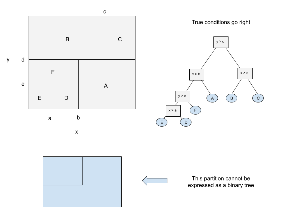
Draw an example of your own invention of a partition of a two–dimensional feature space that could result from a recurive binary splitting. Your example should contain at least six regions. Draw a decision tree corresponding to this partition. Be sure to label all aspects of your figures, including the regions, the cutpoints, and which region corresponds to which leaf of the tree.

(b)

Draw an example of your own invention of a partition of a two–dimensional feature space that could not result from a recurive binary splitting.

Solutions

A possible answer

2 Aggregating bagged classifiers (based on Gareth et al. (2021) 8.4.5)

Suppose we fit classification trees to each of ten bootstrapped datasets containing regressors $\mathit{x}$ and red and green classes. For a particular observation ${\mathit{x}}_n$, each tree gives an estimate of $p(\text{Red}|{\mathit{x}}_n)$, which are:

0.1, 0.15, 0.2, 0.2, 0.55, 0.6, 0.6, 0.65, 0.7, and 0.75.

There are two way to combine these scores to make a single score:

• The majority vote
• Averaging the probabilities, and predicting red if and only if the average probability of red is $>0.5$.

In this example, what is the final classification under these two approaches? Explain any discrepancy in intuitive terms; a single sentence is enough.

Solutions

The classifiers are four green and six red, so the majority vote is red.

The average probability is 0.45, so the average probability approach chooses green.

The difference is due to the fact that though there are fewer green votes, their probability estimates are more extreme.

3 Trees as regression on partition indicators

Suppose $\{A_1,\dots ,A_K\}$ is a partition of ${\mathbb{R}}^P$, meaning $A_k\bigcap A_j=\mathrm{\varnothing }$ for $k\ne j$. Let ${\mathit{x}}_n\in {\mathbb{R}}^P$, and let ${\mathit{z}}_{nk}=\mathrm{I}({\mathit{x}}_n\in A_k)$ denote the indicators of the sets $A_k$, and ${\mathit{z}}_n=({\mathit{z}}_{n1},\dots ,{\mathit{z}}_{nK}{)}^{⊺}$. Finally, let $\mathit{Z}$ denote the $N\times K$ matrix with ${\mathit{z}}_n^{⊺}$ in row $n$, and let $\mathit{Y}=(y_1,\dots ,y_N)$ denote a vector of real–valued responses.

Let $N_k$ denote the number of ${\mathit{x}}_n$ in partition $A_k$, and let ${\overline{y}}_k$ denote the average of the responses $y_n$ in $A_k$: ${\overline{y}}_k=\frac{1}{N_k}\sum _{n:{\mathit{x}}_n\in A_k}{y}_n$.

(a)

Show that ${\mathit{Z}}^{⊺}\mathit{Z}$ is diagonal, with $k$–th diagonal entry equal to $N_k$.

(b)

Let $\hat{\mathit{\beta }}\in {\mathbb{R}}^K$ denote the OLS coefficient from regressing $\mathit{Y}\sim \mathit{Z}\mathit{\beta }$. Show that $\hat{\mathit{\beta }}=({\overline{y}}_1,\dots ,{\overline{y}}_K{)}^{⊺}$.

(c)

Consider a regression tree topology $T$ with leaves $t$; write $t\in T$ for the set of leaves, and write $n\in t$ for the set of observations ${\mathit{x}}_n$ that end up in leaf $t$. Given the tree $T$, suppose we predict a constant $c_t$ for observations $\mathit{x}$ that end up in leaf $t$. Consider the problem of finding the optimal leaf predictions,

$$({\hat{c}}_1,\dots ,{\hat{c}}_{|T|})=\underset{c_t\text{ for }t\in T}{\mathrm{argmin}}\sum _{t\in T}\sum _{n\in t}{(y_n-c_t)}^2.$$

Show directly that the optima are ${\hat{c}}_k={\overline{y}}_k$.

(d)

Show that your result in (c) also follows from (a) and (b). That is, show that the problem of finding the optimal predictions at the leaves of a regression tree is the same as the regression problem in part (b).

(d)

Consider the setting of (c), but for logistic loss. Suppose now that $y_n\in \{0,1\}$, and consider

$$({\hat{c}}_1,\dots ,{\hat{c}}_{|T|})=\underset{c_t\text{ for }t\in T}{\mathrm{argmin}}\sum _{t\in T}\sum _{n\in t}(-y_n\log c_t-(1-y_n)\log (1-c_t)).$$

Show directly that the optima are ${\hat{c}}_k={\hat{\pi }}_k$, where now ${\hat{\pi }}_k$ is the proportion of observations with $y_n=1$ in the leaf.

Solutions

(a)

$z_{nk}=1$ if and only if ${\mathit{x}}_n\in A_k$, so $\sum _{n=1}^N{z}_{nk}=N_k$. And $\sum _{n=1}^N{z}_{nk}{z}_{n{k}^{\prime }}=0$ since each $x_n$ can be in $A_k$, in $A_{k^{\prime }}$, or in neither of them, but not in both, since the sets $A_k$ are a partition. It follows that ${\mathit{Z}}^{⊺}\mathit{Z}$ has the stated form by writing out the matrix multiplication as sums.

(b)

The $k$–th entry of ${\mathit{Z}}^{⊺}\mathit{Y}$ is the sum of $y_n$ among ${\mathit{x}}_n\in A_k$, and $({\mathit{Z}}^{⊺}\mathit{Z}{)}^{-1}$ is diagonal with $1/N_k$ on the diagonal by (a). The result follows from $\hat{\mathit{\beta }}=({\mathit{Z}}^{⊺}\mathit{Z}{)}^{-1}{\mathit{Z}}^{⊺}\mathit{Y}$.

(c)

Each leaf is an indpendent optimization problem, so

$${\hat{c}}_t=\underset{c_t}{\mathrm{argmin}}\sum _{n\in t}{(y_n-c_t)}^2,$$

which we know gives ${\hat{c}}_k={\overline{y}}_k$.

(d)

The tree defines a partition ${\mathit{A}}_t$, where ${\mathit{x}}_n\in {\mathit{A}}_t$ if and only if ${\mathit{x}}_n\in t$ (that is, if ${\mathit{x}}_n$ ends up in leaf $t$ according to the tree topology). In leaf $t$ we predict $c_t$, so our prediction for $y_n$ is $\sum _{t\in T}{\mathit{A}}_t{\text{c}}_t$, and the tree loss can be written equivalently as

$$\sum _{t\in T}\sum _{n\in t}{(y_n-c_t)}^2=\sum _{n=1}^N{(y_n-\sum _{tinT}{\mathit{A}}_t{c}_t)}^2,$$

and the latter is the least squares problem from (a) and (b).

(d)

This can be done either by recognizing that this is logistic regression on indicators, or by observing again that

$${\hat{c}}_t=\underset{c_t}{\mathrm{argmin}}\sum _{n\in t}(-y_n\log c_t-(1-y_n)\log (1-c_t)).$$

The first order condition gives

$$\begin{array}{rl}0=& \frac{-1}{{\hat{c}}_t}\sum _{n\in t}{y}_n+\frac{1}{1-{\hat{c}}_t}\sum _{n\in t}(1-y_n)\\ =& \frac{-1}{{\hat{c}}_t}{N}_t{\hat{\pi }}_t+\frac{1}{1-{\hat{c}}_t}{N}_t(1-{\hat{\pi }}_t)\Rightarrow \\ 0=& (1-{\hat{c}}_t){\hat{\pi }}_t-{\hat{c}}_t(1-{\hat{\pi }}_t)\\ =& {\hat{\pi }}_t-{\hat{c}}_t,\end{array}$$

from which the result follows.

4 Interpretability of regression trees

A commonly claimed advantage of regression trees is their interpretability. That means it can be relatively easy to inspect why a regression tree made the prediction it did. But that does not mean that you can safely use trees to do variable selection for causal inference.

Suppose that you have data that’s generated according to the following process:

$$\begin{array}{rl}z\sim & \mathcal{N}(0,10)\\ x_1|z\sim & \mathcal{N}(z,0.1)\\ x_2|z\sim & \mathcal{N}(z,0.1)\\ y|z=& \mathrm{I}(z>0)\end{array}$$

Suppose we don’t observe $z$, but only observe a random set of $N$ draws $(x_{n1},x_{n2},y_n)$ from this process.

(a)

Suppose we train a regression tree on this data using $x_{n1}$ and $x_{n2}$ as predictors. What is the probability that the variable $x_1$ will be selected for the first split? (Hint: you can argue by symmetry without doing any calculations.)

(b)

Suppose you make the first split on $x_{n1}$. Do you expect subsequent splits on $x_{n2}$ to make large improvements in the fit? (You may argue intuitively, there is no need to do calculations.)

(c)

Suppose you have trained a tree in which $x_{n1}$ is the most important variable, as measured by the average increase in fit within nodes that split on $x_1$. Does this mean that $x_{n2}$, taken alone, is a poor predictor of $y$? Does this mean that $x_{n1}$ is causally related to $y$?

Solutions

(a)

In the data generating process, the stochastic relationship between $x_1$ and $y$ is exactly the same as that between $x_2$ and $y$, so by symmetry the probability of choosing either as the first split is $0.5$.

(b)

Since the variance of $z$ is so much larger than the variance of $x_1|z$, $x_1$ is nearly as good a predictor as $z$ itself, and $x_2$ can provide little extra information. Sometimes when $z$ is very close to $0$, it may be the case that you’d be better off predicting $y=1$ if both $x_1$ and $x_2$ are positive, but this happens rarely. So you will get little predictive benefit from additionally splitting on $x_2$.

(c)

As we’ve seen in (a) and (b), the fact that $x_2$ adds little value once you’ve split on $x_1$ does not mean that $x_2$ is a poor predictor taken alone, nor does it mean that it is causally related. Like L1 regularization, if several explanatory variables are all equally powerful, trees will select one of them and then discard the rest.

5 Monotonic transformations (based on a problem from Erez Buchweitz)

Suppose we are finding the optimal split point for a node $t$ using variable $r_n$. For a split point $\rho$, define

$$\begin{array}{rl}{\overline{y}}_{\rho }^{-}:=& \frac{\sum _{n\in t}\mathrm{I}(r_n<\rho )y_n}{\sum _{n\in t}\mathrm{I}(r_n<\rho )}\\ {\overline{y}}_{\rho }^{+}:=& \frac{\sum _{n\in t}\mathrm{I}(r_n>\rho )y_n}{\sum _{n\in t}\mathrm{I}(r_n>\rho )}\\ R(\rho )=& \sum _{n\in t}((y_n-{\overline{y}}_{\rho }^{-}{)}^2\mathrm{I}(r_n<\rho )+(y_n-{\overline{y}}_{\rho }^{+}{)}^2\mathrm{I}(r_n>\rho )).\end{array}$$

Typically there are a set of $\rho$ that all produce the same value of $R(\rho )$ lying between two datapoints $r_{-}$ and $r_{+}$. Suppose that, when this happens, we always take our split point to be the average, $\hat{\rho }=\frac{1}{2}(r_{+}+r_{-})$

Consider applying CART with the above splitting procedure to regression observations of $({\mathit{x}}_n,y_n)$, and on $({\mathit{z}}_n,y_n)$, where each component of ${\mathit{z}}_n$ is a monotonic transformation of the corresponding component of ${\mathit{x}}_n$. That is, ${\mathit{z}}_{np}={\varphi }_p({\mathit{x}}_{np})$, for each $p$, where ${\varphi }_p$ is either strictly increasing or strictly decreasing.

(a)

In general, will the training error be different for the two datasets? Why or why not?

(b)

In general, will the test error be different for the two datasets? Why or why not?

(c)

Construct a simple one–dimensional example in which one transformation gives a good test set error and the other does not.

Solutions

(a)

The training error will be identical. Since the transformation is either strictly increasing or decreasing, it does not change the sorting of the regressors in any leaf, and so the optimal split points will occur between the same pairs of points, irrespective of whether we split on $\mathit{x}$ or $\mathit{z}$. That is, if we split between ${\mathit{x}}_{np}$ and ${\mathit{x}}_{n{p}^{\prime }}$ at leaf $t$, we will split between on ${\mathit{z}}_{np}$ and ${\mathit{z}}_{n{p}^{\prime }}$ at the same leaf.

(b)

As long as $\varphi$ is non-linear, the test error may be different in general because the actual split points will be different, despite the splits being between the same pairs of datapoints. This is because averages in one space are not the same as averages in the other. Formally, you might say that:

$$\frac{1}{2}({\mathit{x}}_{np}+{\mathit{x}}_{n{p}^{\prime }})=\frac{1}{2}({\varphi }^{-1}(\varphi ({\mathit{x}}_{np}))+{\varphi }^{-1}(\varphi ({\mathit{x}}_{n{p}^{\prime }})))=\frac{1}{2}({\varphi }^{-1}({\mathit{z}}_{np})+{\varphi }^{-1}({\mathit{z}}_{n{p}^{\prime }}))\ne {\varphi }^{-1}(\frac{1}{2}({\mathit{z}}_{np}+{\mathit{z}}_{n{p}^{\prime }})).$$

(c)

Suppose that we have two points, $x_1=-10$ and $x_2=10$, and $y=\mathrm{I}(x>0)$. A classifier on $x$ splits at $\frac{1}{2}(-10+10)=0$ which is the optimal point. But if we take $z=\exp (x)$, which is strictly increasing, then we split at $\frac{1}{2}(\exp (-10)+\exp (10))\approx 11013$, which corresponds to $x=\log (11013)=9.3$, a terrible split point.

$$$$

6 The accuracy of bagging (based on Bühlmann and Yu (2002)) (254 only $\star$ $\star$ $\star$)

In this problem we explore some simple settings in which bagging does and does not work.

(a)

Suppose we observe $\mathit{Y}=(y_1,\dots ,y_N{)}^{⊺}$, which we use to fit the constant model, $f={\beta }_0$. We use least squares regression, so ${\hat{\beta }}_0=\frac{1}{N}\sum _{n=1}^N{y}_n$, and so $\hat{f}=\frac{1}{N}\sum _{n=1}^N{y}_n$.

Let ${\mathit{Y}}^{\ast }=(y_1^{\ast },\dots ,y_N^{\ast }{)}^{⊺}$ denote a bootstrap sample from $\mathit{Y}$, and write the ideal bagging estimator as

$${\hat{f}}^{\ast }={\mathbb{E}}_{{\mathit{Y}}^{\ast }}\left[\frac{1}{N}\sum _{n=1}^N{y}_n^{\ast }\right].$$

Show that ${\hat{f}}^{\ast }=\hat{f}$. That is, bagging does not improve the estimator in this case. In fact, it makes it worse if ${\hat{f}}^{\ast }$ is estimated using a finite number of bootstrap samples, since it increases the variance due to the bootstrap Monte Carlo sampling.

(b)

Next, suppose that we observe pairs $(x_n,y_n)$, where $x_n\sim \mathcal{N}(\mu ,1)$ and $y_n\in \{0,1\}$. Writing $\mathit{X}$ for the vectors of observations, suppose that we wish to predict $y_n$ from $x_n$ using the following classifier:

$$\hat{f}(x;\mathit{X})=\mathrm{I}(x\ge \frac{1}{N}\sum _{n=1}^N{x}_n).$$

Let $\mathrm{\Phi }(\cdot )$ denote the CDF of the standard normal distribution. Show that, for a fixed $x$,

$$\begin{array}{rl}{\mathbb{E}}_{\mathit{X}}[\hat{f}(x;\mathit{X})]=& \mathrm{\Phi }(\sqrt{N}(x-\mu ))\\ {\mathrm{Var}}_{\mathit{X}}(\hat{f}(x;\mathit{X}))=& \mathrm{\Phi }(\sqrt{N}(x-\mu ))(1-\mathrm{\Phi }(\sqrt{N}(x-\mu ))).\end{array}$$

(c)

In the setting of (b), let ${\mathit{X}}^{\ast }$ denote a bootstrap sample from $\mathit{X}$.
Let $\overline{x}=\frac{1}{N}\sum _{n=1}^N{x}_n$. Using this, show that the bagged estimator for a fixed $x$ and large $N$ is

$$\begin{array}{rl}{\hat{f}}^{\ast }(x;\mathit{X})\approx & \mathrm{\Phi }(\sqrt{N}(x-\overline{x})).\end{array}$$

Note that the bagged estimator replaced a sharp threshold $\hat{f}(x;\mathit{X})=\mathrm{I}(x\ge \overline{x})$ with a soft threshold ${\hat{f}}^{\ast }(x;\mathit{X})\approx \mathrm{\Phi }(\sqrt{N}(x-\overline{x}))$.

Hint: Under the bootstrap distribution, you may use without proof the fact that, for large $N$, $\sqrt{N}(\frac{1}{N}\sum _{n=1}^N{x}_n^{\ast }-\overline{x})\approx \mathcal{N}(0,1)$ under the bootstrap randomness. (Note that in the bootstrap sampling distribution, $\overline{x}$ is fixed.)

(d)

Evaluating the result for (b) and (c) at $x=\mu$, show that, for large $N$,

$$\begin{array}{rlrl}{\mathbb{E}}_{\mathit{X}}[{\hat{f}}^{\ast }(x;\mathit{X})]\approx & \frac{1}{2}& {\mathbb{E}}_{\mathit{X}}[\hat{f}(x;\mathit{X})]=& \frac{1}{2}\\ {\mathrm{Var}}_{\mathit{X}}({\hat{f}}^{\ast }(x;\mathit{X}))\approx & \frac{1}{12}& {\mathrm{Var}}_{\mathit{X}}(\hat{f}(x;\mathit{X}))=& \frac{1}{4}.\end{array}$$

Conclude that, for $x=\mu$, the bagged estimator maintains the same expected prediction function, but reduces the variance by a factor of $3$.

Hint: use the fact that $\sqrt{N}(\mu -\overline{x})$ is a standard normal, and that $\mathrm{\Phi }(Z)$ is uniform if $Z\sim \mathcal{N}(0,1)$.

Solutions

(a)

This was done in lecture.

(b)

By normality, $\frac{1}{N}\sum _{n=1}^N{x}_n\sim \mathcal{N}(\mu ,N^{-1})$, so $\sqrt{N}(\frac{1}{N}\sum _{n=1}^N{x}_n-\mu )\sim \mathcal{N}(0,1)$. Let $z\sim \mathcal{N}(0,1)$. Then

$$\begin{array}{rl}{\mathbb{E}}_{\mathit{X}}[\hat{f}(x;\mathit{X})]=& {\mathbb{P}}_{}(x\ge \frac{1}{N}\sum _{n=1}^N{x}_n)\\ =& {\mathbb{P}}_{}(\sqrt{N}(x-\mu )\ge z)\\ =& \mathrm{\Phi }(\sqrt{N}(x-\mu )).\end{array}$$

Since $\mathrm{I}(x\ge \frac{1}{N}\sum _{n=1}^N{x}_n)$ is a binary variable, with expectation $p=\mathrm{\Phi }(\sqrt{N}(x-\mu ))$, its variance is $p(1-p)$, and plugging in gives the desired answer.

(c)

The reasoning is as in (b) but using the CLT applied to the bootstrap distribution.

$$\begin{array}{rl}{\hat{f}}^{\ast }(x;\mathit{X})=& {\mathbb{E}}_{{\mathit{X}}^{\ast }}[{\hat{f}}^{\ast }(x;{\mathit{X}}^{\ast })]\\ =& {\mathbb{E}}_{{\mathit{X}}^{\ast }}\left[\mathrm{I}(x\ge \frac{1}{N}\sum _{n=1}^N{x}_n^{\ast })\right]\\ =& {\mathbb{E}}_{{\mathit{X}}^{\ast }}\left[\mathrm{I}(\sqrt{N}(x-\overline{x})\ge \sqrt{N}(\frac{1}{N}\sum _{n=1}^N{x}_n^{\ast }-\overline{x}))\right]\\ \approx & {\mathbb{E}}_{{\mathit{X}}^{\ast }}\left[\mathrm{I}(\sqrt{N}(x-\overline{x})\ge Z)\right]\\ =& \mathrm{\Phi }(\sqrt{N}(x-\overline{x})).\end{array}$$

(d)

Evaluating the result for (b) and (c) at $x=\mu$, show that

$$\begin{array}{rl}{\mathbb{E}}_{\mathit{X}}[{\hat{f}}^{\ast }(x;\mathit{X})]=& {\mathbb{E}}_{\mathit{X}}[\mathrm{\Phi }(\sqrt{N}(\mu -\overline{x}))]\\ =& {\mathbb{E}}_{\mathit{X}}[\mathrm{\Phi }(Z)]\\ =& {\int }_0^{1}udu\\ =& \frac{1}{2}.\end{array}$$

and

$$\begin{array}{rl}{\mathrm{Var}}_{\mathit{X}}({\hat{f}}^{\ast }(x;\mathit{X}))=& {\int }_0^1{u}^{2}du-\frac{1}{4}\\ =& \frac{1}{3}-\frac{1}{4}\\ =& \frac{1}{12}.\end{array}$$

7 Trees as approximations to linear functions (254 only $\star$ $\star$ $\star$)

Suppose you are trying to use a regression tree to represent the function $y={\mathbb{E}}_{}[y|x]:=f(x)=x$ for $x\in {\mathbb{R}}^{}$. That is, $y$ is observed without noise and the regression function is linear, but we’re approximating the linear function with a decision tree. Assume that $x$ is uniformly distributed on $[0,1]$.

(a)

Consider a connected set $A$ with endpoints $A_L$ and $A_R$ (i.e. $A=\{x:A_L\le \mathit{X}<A_R\}$), and let $\mathrm{\Delta }=A_R-A_L$ denote the width of $A$.

Suppose we predict $y_A^{\ast }$ for $x\in A$, where $y_A^{\ast }=\underset{c}{\mathrm{argmin}}{\int }_A(f(x)-c{)}^{2}dx$ is the ideal least squares estimator in the set $A$. Show that $y_A^{\ast }=\frac{1}{2}(A_L+A_R)$, and that the integrated error is

$${\int }_A(f(x)-y_A^{\ast }{)}^{2}dx=\frac{{\mathrm{\Delta }}^3}{12}.$$

(b)

Suppose we partition the unit interval into $K$ equally spaced intervals, each with width $1/K$, with indicator functions $A_k$. Suppose we find the optimal least–squares prediction $y^{\ast }(x)$ for the regression of $y$ on these indicators. Using (a), find an expression for the expected squared error ${\mathbb{E}}_{x,y}[(y-y^{\ast }(x){)}^2]$ as a function of $K$.

(c)

In the setting of (b), for a fixed $\epsilon >0$, how large do we need to make $K$ in order to acheive ${\mathbb{E}}_{x,y}[(y-y^{\ast }(x){)}^2]\le \epsilon$?

(d)

Suppose we grow a regression tree with depth $D$, where each branch is split at the optimal point in the middle of the parent’s interval. For a fixed $\epsilon >0$, how large do we need to make $D$ in order to acheive ${\mathbb{E}}_{x,y}[(y-y^{\ast }(x){)}^2]\le \epsilon$?

Note: It seems to me that computer scientists love to do accuracy order calculations like this!

Solutions

(a)

All we really need is the two integrals

$$\begin{array}{rl}{\int }_a^{b}xdx=& \frac{1}{2}{\left[x^2\right]}_a^b=\frac{1}{2}(b^2-a^2)\text{ and}\\ {\int }_a^b{x}^{2}dx=& \frac{1}{3}{\left[x^3\right]}_a^b=\frac{1}{3}(b^3-a^3).\end{array}$$

We know that $y_A^{\ast }$ satisfies the first–order condition

$$\frac{\partial }{\partial c}{\int }_A(f(x)-c{)}^{2}dx=-2{\int }_A(f(x)-c)dx=0$$

so $$\begin{array}{rl}{y}_A^{\ast }=& \frac{{\int }_{A}f(x)dx}{{\int }_{A}dx}\\ =& \frac{\frac{1}{2}(A_R^2-A_L^2)}{A_R-A_L}\\ =& \frac{1}{2}(A_R+A_L).\end{array}$$

A simple way to do the second integral is to note that ${\int }_0^1(x-1/2{)}^{2}dx=\frac{1}{12}$, so that ${\int }_0^1(\mathrm{\Delta }x-A_L-(\mathrm{\Delta }/2+A_L){)}^{2}dx=\frac{{\mathrm{\Delta }}^2}{12}$. Making the subsititution $z=\mathrm{\Delta }x-A_L$ into the integral gives the desired result.

(b)

$$\begin{array}{rl}{\mathbb{E}}_{x,y}[(y-y^{\ast }(x){)}^2]=& {\mathbb{E}}_x[\sum _{k=1}^K\mathrm{I}(\frac{k-1}{K}<x<\frac{k}{K})(x-y^{\ast }(x){)}^2]\\ =& \sum _{k=1}^K{\int }_{(k-1)/K}^{k/K}{(x-y_k^{\ast })}^{2}dx\\ =& K\frac{1}{12K^3}\\ =& \frac{1}{12K^2},\end{array}$$

where we used (a) in the second-to-last line.

(c)

By (b) we require

$$\frac{1}{12K^2}\le \epsilon \iff K\ge \frac{1}{\sqrt{12\epsilon }}.$$

Since $K$ must be an integer, we can take $K=\lceil \frac{1}{\sqrt{12\epsilon }}\rceil$.

(d)

The optimal split point is always in the middle of the interval, so if we have a tree of depth $D$ then we have a partition into $K=2^D$ regions. (Here I take a depth one tree to be a single split, but the question is ambiguous, and taking a depth one tree to be a single node is also fine, in which case you get $K=2^{D-1}$.)

By (c) we then require

$$2^D=\exp (D\log (2))\ge \frac{1}{\sqrt{12\epsilon }}\iff D\ge \frac{\log (-12\epsilon )}{\log (2)}.$$

Again, $D$ must be an integer, so we can take $D=\lceil \frac{\log (-12\epsilon )}{\log (2)}\rceil$.

8 Bibliography

Bühlmann, Peter, and Bin Yu. 2002. “Analyzing bagging.” The Annals of Statistics 30 (4): 927–61. https://doi.org/10.1214/aos/1031689014.

Gareth, J., W. Daniela, H. Trevor, and T. Robert. 2021. An Introduction to Statistical Learning: With Applications in Python. Spinger.