import pandas as pd
import numpy as np
from matplotlib import pyplot as pltLab 10 Presentation - Third Competition Round-Up
1 Prepare simulation setup
Here’s how one could approach the competition.
1.1 Load data
dir_path = r"../datasets/competition_3_diabetes/"
X = pd.read_parquet(f"{dir_path}X_train.parquet")
y = pd.read_parquet(f"{dir_path}y_train.parquet").squeeze()
X.shape, y.shape
((200000, 21), (200000,))1.2 Cross validation folds
Split randomly into five folds.
nfolds = 5
fold = np.resize(list(range(nfolds)), X.shape[0])
np.random.shuffle(fold)
cv_pairs = [{
    "X_train": X.loc[fold != i,:],
    "y_train": y.loc[fold != i],
    "X_valid": X.loc[fold == i,:],
    "y_valid": y.loc[fold == i],
    } for i in np.unique(fold)
]
[(entry["X_train"].shape[0], entry["X_valid"].shape[0]) for entry in cv_pairs]
[(160000, 40000),
(160000, 40000),
(160000, 40000),
(160000, 40000),
(160000, 40000)]1.3 Cross validation workflow
Here is a basic workflow that does:
- Train model on trainset
- Tune threshold (how?)
- Score on validset
from sklearn.metrics import f1_score, precision_recall_curve

def fit_predict_score(X_train, y_train, X_valid, y_valid, model, in_sample=False):
    model.fit(X_train, y_train)
    thresh = find_best_threshold(y_train, predict(model, X_train))
    if in_sample:
        pred = predict(model, X_train) > thresh
        return f1_score(y_train, pred)
    else:
        pred = predict(model, X_valid) > thresh
        return f1_score(y_valid, pred)


def predict(model, X):
    if hasattr(model, "predict_proba"):
        return model.predict_proba(X)[:,1]
    elif hasattr(model, "decision_function"):
        return model.decision_function(X)
    else:
        return model.predict(X)

def find_best_threshold(y, pred):
    precision, recall, thresholds = precision_recall_curve(y, pred)
    f1 = 2 * precision * recall / np.where(precision + recall == 0, 1, precision + recall)
    idx = np.argmax(f1)
    return thresholds[idx]

def cv_workflow(model, **kwargs):
    scores = [fit_predict_score(model=model, **entry, **kwargs) for entry in cv_pairs]
    return np.mean(scores)
1.4 Tuning the threshold
A few options:
- Tune on trainset (like the code above)
- Tune on validset (like many of you did)
- Split thresholdset from trainset and tune on it
- Treat as any other hyperparameter and train model for each threshold value
Question: what are the pros and cons of each method?
Answer:
- Tune on trainset - overfitting threshold
- Tune on validset - biasing the cross validation
- Tune on thresholdset - fewer observations to train on
- Retrain for each threshold - computationally intensive
1.5 Test run
Let’s train simple models.
from sklearn.linear_model import LogisticRegression, Lasso
from sklearn.discriminant_analysis import LinearDiscriminantAnalysis
from sklearn.svm import LinearSVC
from sklearn.preprocessing import StandardScaler
from sklearn.pipeline import Pipeline
from datetime import datetime

predictors = {
    "logistic": LogisticRegression(C=10000000000),
    "lasso": Lasso(alpha=0.0001),
    "lda": LinearDiscriminantAnalysis(shrinkage=0, solver="lsqr"),
    "svm": LinearSVC(C=0.00001, dual="auto"),
}
for nm, predictor in predictors.items():
    model = Pipeline([
        ("scaler", StandardScaler()),
        ("predictor", predictor),
    ])
    score = cv_workflow(model)
    print(f"[{datetime.now().strftime('%Y-%m-%d %H:%M:%S')}] {nm}={score}")
print(f"[{datetime.now().strftime('%Y-%m-%d %H:%M:%S')}] end")
[2025-04-04 12:51:01] logistic=0.4614040229289825
[2025-04-04 12:51:04] lasso=0.45799255247438725
[2025-04-04 12:51:06] lda=0.45804499442409535
[2025-04-04 12:51:11] svm=0.45555107822384766
[2025-04-04 12:51:11] endQuestion: are these good scores?
Answer: the answer is data dependent, on some datasets you cannot do better than this. Is this one of those datasets?
Add to backlog:
- Try tuning threshold on thresholdset.
2 Tune regularization penalty
Logistic:
predictors = {
    C: LogisticRegression(C=C)
    for C in [1, 100, 1000, 1000000, 1000000, 100000000, 10000000000]
}
for nm, predictor in predictors.items():
    model = Pipeline([
        ("scaler", StandardScaler()),
        ("predictor", predictor),
    ])
    score = cv_workflow(model)
    print(f"[{datetime.now().strftime('%Y-%m-%d %H:%M:%S')}] {nm}={score}")
print(f"[{datetime.now().strftime('%Y-%m-%d %H:%M:%S')}] end")
[2025-04-04 12:51:13] 1=0.4612578742987442
[2025-04-04 12:51:16] 100=0.4614040229289825
[2025-04-04 12:51:19] 1000=0.4614040229289825
[2025-04-04 12:51:22] 1000000=0.4614040229289825
[2025-04-04 12:51:24] 100000000=0.4614040229289825
[2025-04-04 12:51:27] 10000000000=0.4614040229289825
[2025-04-04 12:51:27] endSVM:
predictors = {
    C: LinearSVC(C=C, dual="auto")
    for C in [0.000001, 0.00001, 0.0001, 0.001, 0.01, 0.1, 1]
}
for nm, predictor in predictors.items():
    model = Pipeline([
        ("scaler", StandardScaler()),
        ("predictor", predictor),
    ])
    score = cv_workflow(model)
    print(f"[{datetime.now().strftime('%Y-%m-%d %H:%M:%S')}] {nm}={score}")
print(f"[{datetime.now().strftime('%Y-%m-%d %H:%M:%S')}] end")
[2025-04-04 12:51:31] 1e-06=0.4393943583018654
[2025-04-04 12:51:35] 1e-05=0.45555107822384766
[2025-04-04 12:51:40] 0.0001=0.4602461324011517
[2025-04-04 12:51:45] 0.001=0.4601514982969565
[2025-04-04 12:51:50] 0.01=0.46115568232964793
[2025-04-04 12:51:55] 0.1=0.46119812173261154
[2025-04-04 12:52:01] 1=0.4612184250879605
[2025-04-04 12:52:01] endLasso:
predictors = {
    alpha: Lasso(alpha=alpha)
    for alpha in [0.00000000001, 0.0000001, 0.000001, 0.0001, 0.0001, 0.001, 0.01, 0.1, 1]
}
for nm, predictor in predictors.items():
    model = Pipeline([
        ("scaler", StandardScaler()),
        ("predictor", predictor),
    ])
    score = cv_workflow(model)
    print(f"[{datetime.now().strftime('%Y-%m-%d %H:%M:%S')}] {nm}={score}")
print(f"[{datetime.now().strftime('%Y-%m-%d %H:%M:%S')}] end")
[2025-04-04 12:52:05] 1e-11=0.45804499442409535
[2025-04-04 12:52:08] 1e-07=0.45804499442409535
[2025-04-04 12:52:11] 1e-06=0.4580002367039159
[2025-04-04 12:52:13] 0.0001=0.45799255247438725
[2025-04-04 12:52:15] 0.001=0.45753509833651657
[2025-04-04 12:52:17] 0.01=0.4551825718127631
[2025-04-04 12:52:19] 0.1=0.1935941506689048
[2025-04-04 12:52:20] 1=0.0
[2025-04-04 12:52:20] endLDA:
predictors = {
    shrinkage: LinearDiscriminantAnalysis(shrinkage=shrinkage, solver="lsqr")
    for shrinkage in [i/10 for i in range(11)]
}
for nm, predictor in predictors.items():
    model = Pipeline([
        ("scaler", StandardScaler()),
        ("predictor", predictor),
    ])
    score = cv_workflow(model)
    print(f"[{datetime.now().strftime('%Y-%m-%d %H:%M:%S')}] {nm}={score}")
print(f"[{datetime.now().strftime('%Y-%m-%d %H:%M:%S')}] end")
[2025-04-04 12:52:22] 0.0=0.45804499442409535
[2025-04-04 12:52:25] 0.1=0.45702907101108553
[2025-04-04 12:52:27] 0.2=0.45600224466717665
[2025-04-04 12:52:29] 0.3=0.4535600149629473
[2025-04-04 12:52:32] 0.4=0.45137167825646324
[2025-04-04 12:52:34] 0.5=0.4481299848718205
[2025-04-04 12:52:36] 0.6=0.4454134544472283
[2025-04-04 12:52:38] 0.7=0.4421960275675084
[2025-04-04 12:52:40] 0.8=0.4397890893151556
[2025-04-04 12:52:42] 0.9=0.43548647043119815
[2025-04-04 12:52:44] 1.0=0.4307984696857252
[2025-04-04 12:52:44] end3 Do we need more expressivity?
Let’s compute losses in and out of sample.
predictors = {
    "logistic": LogisticRegression(C=1),
    "lasso": Lasso(alpha=0.000001),
    "lda": LinearDiscriminantAnalysis(shrinkage=0, solver="lsqr"),
    "svm": LinearSVC(C=0.01, dual="auto"),
}
for nm, predictor in predictors.items():
    model = Pipeline([
        ("scaler", StandardScaler()),
        ("predictor", predictor),
    ])
    score = cv_workflow(model)
    score_in_sample = cv_workflow(model, in_sample=True)
    print(f"[{datetime.now().strftime('%Y-%m-%d %H:%M:%S')}] {nm}={score} ({score_in_sample})")
print(f"[{datetime.now().strftime('%Y-%m-%d %H:%M:%S')}] end")
[2025-04-04 12:52:50] logistic=0.4612578742987442 (0.4622458870106123)
[2025-04-04 12:52:56] lasso=0.4580002367039159 (0.4591032959852958)
[2025-04-04 12:53:01] lda=0.45804499442409535 (0.4591019048572953)
[2025-04-04 12:53:12] svm=0.46115568232964793 (0.4620955920215676)
[2025-04-04 12:53:12] endLooks like regularization is not helpful at this point.
3.1 Feature engineering
Let’s look at the features.
{col: str(np.sort(X[col].unique()).tolist()) for col in X.columns}{'HighBP': '[0, 1]',
'HighChol': '[0, 1]',
'CholCheck': '[0, 1]',
'BMI': '[12, 13, 14, 15, 16, 17, 18, 19, 20, 21, 22, 23, 24, 25, 26, 27, 28, 29, 30, 31, 32, 33, 34, 35, 36, 37, 38, 39, 40, 41, 42, 43, 44, 45, 46, 47, 48, 49, 50, 51, 52, 53, 54, 55, 56, 57, 58, 59, 60, 61, 62, 63, 64, 65, 66, 67, 68, 69, 70, 71, 72, 73, 74, 75, 76, 77, 78, 79, 80, 81, 82, 83, 84, 86, 87, 88, 89, 90, 91, 92, 95, 96, 98]',
'Smoker': '[0, 1]',
'Stroke': '[0, 1]',
'HeartDiseaseorAttack': '[0, 1]',
'PhysActivity': '[0, 1]',
'Fruits': '[0, 1]',
'Veggies': '[0, 1]',
'HvyAlcoholConsump': '[0, 1]',
'AnyHealthcare': '[0, 1]',
'NoDocbcCost': '[0, 1]',
'GenHlth': '[1, 2, 3, 4, 5]',
'MentHlth': '[0, 1, 2, 3, 4, 5, 6, 7, 8, 9, 10, 11, 12, 13, 14, 15, 16, 17, 18, 19, 20, 21, 22, 23, 24, 25, 26, 27, 28, 29, 30]',
'PhysHlth': '[0, 1, 2, 3, 4, 5, 6, 7, 8, 9, 10, 11, 12, 13, 14, 15, 16, 17, 18, 19, 20, 21, 22, 23, 24, 25, 26, 27, 28, 29, 30]',
'DiffWalk': '[0, 1]',
'Sex': '[0, 1]',
'Age': '[1, 2, 3, 4, 5, 6, 7, 8, 9, 10, 11, 12, 13]',
'Education': '[1, 2, 3, 4, 5, 6]',
'Income': '[1, 2, 3, 4, 5, 6, 7, 8]'}There appear to be some numeric features, and most of the rest are binary. Let’s create lists of each kind.
features_binary = [col for col in X.columns if X[col].nunique() == 2]
features_numeric = [col for col in X.columns if X[col].nunique() > 2]
features_numeric, features_binary
(['BMI', 'GenHlth', 'MentHlth', 'PhysHlth', 'Age', 'Education', 'Income'],
['HighBP',
'HighChol',
'CholCheck',
'Smoker',
'Stroke',
'HeartDiseaseorAttack',
'PhysActivity',
'Fruits',
'Veggies',
'HvyAlcoholConsump',
'AnyHealthcare',
'NoDocbcCost',
'DiffWalk',
'Sex'])3.2 Numeric features
3.2.1 Quantile plot for logistic regression
Here is a variant of quantile plot for logistic regression, that applies logistic transform to the mean y values. Remember that logistic regression assumes: \[
\log\left(\frac{p}{1-p}\right) = \boldsymbol{x}^T\boldsymbol{\beta}
\] where \(p=\mathbb{P}(y=1|\boldsymbol{x})\).
So we will apply the same transformation to the average \(y\) values in each bin, and we’ll want to make like transformed line as linear as possible.
def quantile_plot(x, y, by=None, bins=10, by_bins=3, y_fn=lambda x: x):
    assert len(x) == len(y)

    def qp_data(x, y):
        fac = np.searchsorted(np.quantile(x, q=[i / bins for i in range(1, bins)]), x)
        ufac = np.unique(fac)
        qx = np.array([np.mean(x[fac == f]) for f in ufac])
        qy = np.array([y_fn(np.mean(y[fac == f])) for f in ufac])
        return qx, qy

    qx, qy = qp_data(x, y)
    if by is None:
        plt.plot(qx, qy, "-o")
    else:
        assert len(x) == len(by)
        plt.plot(qx, qy, "-o", label="ALL", color="lightgrey")
        by_fac = np.searchsorted(np.quantile(by, q=[i / by_bins for i in range(1, by_bins)]), by)
        by_ufac = np.unique(by_fac)
        for i, f in enumerate(np.unique(by_ufac)):
            mask = by_fac == f
            nm = f"{i}) {min(by[mask]):.2f} / {max(by[mask]):.2f}"
            qx, qy = qp_data(x[mask], y[mask])
            plt.plot(qx, qy, "-o", label=nm)
        plt.legend()

def quantile_plot_logistic(*args, **kwargs):
    quantile_plot(*args, y_fn=lambda x: np.log(x / (1 - x)), **kwargs)
Now to plot all numeric features:
for feature in features_numeric:
    plt.figure()
    quantile_plot_logistic(X[feature], y, bins=100)
    plt.title(feature)
    plt.show()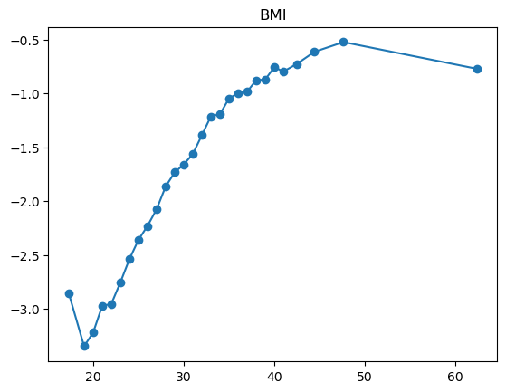
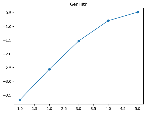
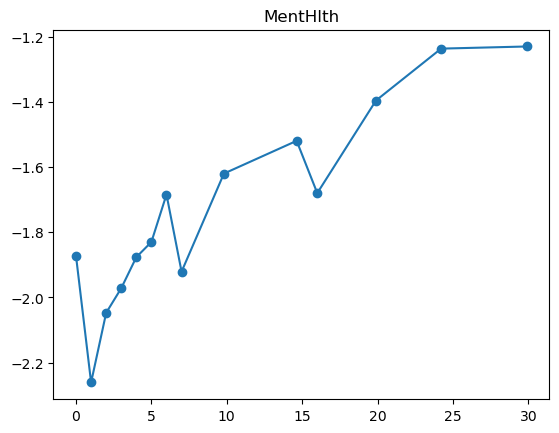
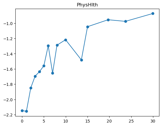
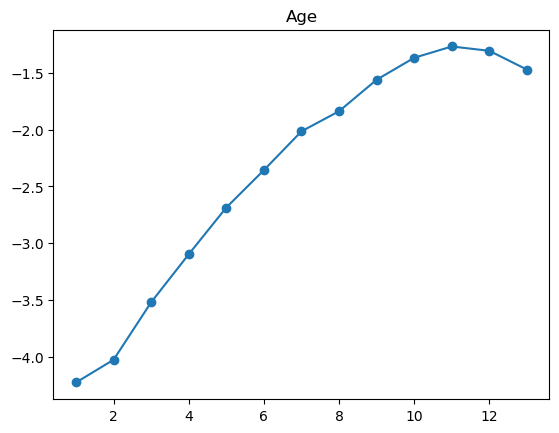
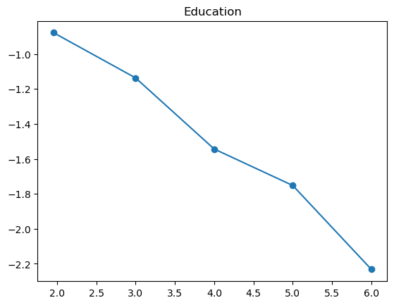
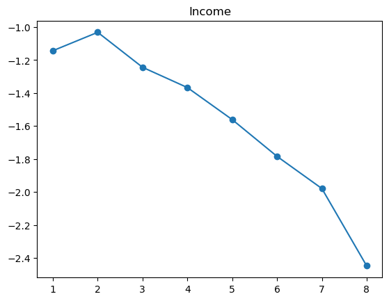
For some of the features (BMI, age, income), the shape looks completely believable (remember we have lots of data). We might be tempted to just throw in a very expressive transformation, say cubic spline with 20 knots, and see what happens. Let’s try that.
3.2.2 Expressive transformation to numeric features
from sklearn.preprocessing import SplineTransformer
from sklearn.compose import ColumnTransformer

predictors = {
    "logistic": LogisticRegression(C=1),
    "lasso": Lasso(alpha=0.01),
    "lda": LinearDiscriminantAnalysis(shrinkage=0, solver="lsqr"),
    "svm": LinearSVC(C=0.01, dual="auto"),
}
print(f"[{datetime.now().strftime('%Y-%m-%d %H:%M:%S')}] end")
for nm, predictor in predictors.items():
    transformer_numeric = Pipeline(steps=[
        ('spline', SplineTransformer(degree=3, n_knots=20)),
        ('scaler', StandardScaler())
    ])
    transformer_binary = Pipeline(steps=[
        ('scaler', StandardScaler())
    ])
    preprocessor = ColumnTransformer(
        transformers=[
            ('numeric', transformer_numeric, features_numeric),
            ('binary', transformer_binary, features_binary)
        ]
    )
    model = Pipeline([
        ("preprocessor", preprocessor),
        ("predictor", predictor),
    ])
    score = cv_workflow(model)
    print(f"[{datetime.now().strftime('%Y-%m-%d %H:%M:%S')}] {nm}={score}")
print(f"[{datetime.now().strftime('%Y-%m-%d %H:%M:%S')}] end")
[2025-04-04 12:53:42] logistic=0.4690488043555326
[2025-04-04 12:54:10] lasso=0.45330544429073233
[2025-04-04 12:54:35] lda=0.459476711550418
[2025-04-04 12:56:30] svm=0.4674114099163023
[2025-04-04 12:56:30] endNumber of features:
len(model.named_steps['preprocessor'].get_feature_names_out())168Add to backlog:
- Less expressive transformation for features that don’t appear to deserve it.
- Add interactions.
3.3 Binary features
Any transformation to a binary feature is an affine transformation, which doesn’t affect a linear model (apart from possibly penalizing the feature differently).
Let’s try to add interactions and see what happens.
from sklearn.preprocessing import PolynomialFeatures

predictors = {
    "logistic": LogisticRegression(C=1),
    #"lasso": Lasso(alpha=0.01),
    "lda": LinearDiscriminantAnalysis(shrinkage=0, solver="lsqr"),
    "svm": LinearSVC(C=0.01, dual="auto"),
}
print(f"[{datetime.now().strftime('%Y-%m-%d %H:%M:%S')}] start")
for nm, predictor in predictors.items():
    transformer_numeric = Pipeline(steps=[
        ('spline', SplineTransformer(degree=3, n_knots=20)),
        ('scaler', StandardScaler())
    ])
    transformer_binary = Pipeline(steps=[
        ('poly', PolynomialFeatures(degree=2, interaction_only=True, include_bias=False)),
        ('scaler', StandardScaler())
    ])
    preprocessor = ColumnTransformer(
        transformers=[
            ('numeric', transformer_numeric, features_numeric),
            ('binary', transformer_binary, features_binary)
        ]
    )
    model = Pipeline([
        ("preprocessor", preprocessor),
        ("predictor", predictor),
    ])
    score = cv_workflow(model)
    print(f"[{datetime.now().strftime('%Y-%m-%d %H:%M:%S')}] {nm}={score}")
print(f"[{datetime.now().strftime('%Y-%m-%d %H:%M:%S')}] end")
[2025-04-04 13:50:03] start
[2025-04-04 13:50:49] logistic=0.47084598935372934
[2025-04-04 13:51:10] lda=0.46446677312539686
[2025-04-04 13:53:34] svm=0.46995657867346646
[2025-04-04 13:53:34] end4 Retune regularization
predictors = {
    C: LinearSVC(C=C, dual="auto")
    for C in [0.000001, 0.00001, 0.0001, 0.001, 0.01]
}
print(f"[{datetime.now().strftime('%Y-%m-%d %H:%M:%S')}] start")
for nm, predictor in predictors.items():
    transformer_numeric = Pipeline(steps=[
        ('spline', SplineTransformer(degree=3, n_knots=20)),
        ('scaler', StandardScaler())
    ])
    transformer_binary = Pipeline(steps=[
        ('poly', PolynomialFeatures(degree=2, interaction_only=True, include_bias=False)),
        ('scaler', StandardScaler())
    ])
    preprocessor = ColumnTransformer(
        transformers=[
            ('numeric', transformer_numeric, features_numeric),
            ('binary', transformer_binary, features_binary)
        ]
    )
    model = Pipeline([
        ("preprocessor", preprocessor),
        ("predictor", predictor),
    ])
    score = cv_workflow(model)
    print(f"[{datetime.now().strftime('%Y-%m-%d %H:%M:%S')}] {nm}={score}")
print(f"[{datetime.now().strftime('%Y-%m-%d %H:%M:%S')}] end")
[2025-04-04 13:54:11] start
[2025-04-04 13:54:36] 1e-06=0.4544754791334615
[2025-04-04 13:55:14] 1e-05=0.4630177566185475
[2025-04-04 13:56:07] 0.0001=0.4671811106134466
[2025-04-04 13:57:47] 0.001=0.46953948020749225
[2025-04-04 14:00:12] 0.01=0.46995657867346646
[2025-04-04 14:00:12] endInteractions for binary features helps slightly, but this increases running time. Regularization is still not needed Number of features:
len(model.named_steps['preprocessor'].get_feature_names_out())2595 Ensembling
Let’s try averaging the three models. First, define the models.
predictors = {
    "logistic": LogisticRegression(C=1),
    "lasso": Lasso(alpha=0.1),
    "lda": LinearDiscriminantAnalysis(shrinkage=0, solver="lsqr"),
    "svm": LinearSVC(C=0.01, dual="auto"),
}
transformer_numeric = Pipeline(steps=[
    ('spline', SplineTransformer(degree=3, n_knots=20)),
    ('scaler', StandardScaler())
])
transformer_binary = Pipeline(steps=[
    ('poly', PolynomialFeatures(degree=2, interaction_only=True, include_bias=False)),
    ('scaler', StandardScaler())
])
preprocessor = ColumnTransformer(
    transformers=[
        ('numeric', transformer_numeric, features_numeric),
        ('binary', transformer_binary, features_binary)
    ]
)
models = {
    nm: Pipeline([
        ("preprocessor", preprocessor),
        ("predictor", predictor),
    ])
    for nm, predictor in predictors.items()
}
Single train-valid-test split.
X_train, y_train, X_valid, y_valid = cv_pairs[0]["X_train"], cv_pairs[0]["y_train"], cv_pairs[0]["X_valid"], cv_pairs[0]["y_valid"]print(f"[{datetime.now().strftime('%Y-%m-%d %H:%M:%S')}] start")
for nm, model in models.items():
model.fit(X_train, y_train)
print(f"[{datetime.now().strftime('%Y-%m-%d %H:%M:%S')}] {nm}")
print(f"[{datetime.now().strftime('%Y-%m-%d %H:%M:%S')}] end")[2025-04-04 14:02:26] start
[2025-04-04 14:02:33] logistic
[2025-04-04 14:02:36] lasso
[2025-04-04 14:02:39] lda
[2025-04-04 14:03:08] svm
[2025-04-04 14:03:08] endpreds = {nm: predict(model, X_train) for nm, model in models.items()}
locs = {nm: pred.mean() for nm, pred in preds.items()}
scales = {nm: pred.std() for nm, pred in preds.items()}
preds_normalized = {nm: (pred - locs[nm]) / scales[nm] for nm, pred in preds.items()}
preds_valid_normalized = {nm: (predict(model, X_valid) - locs[nm]) / scales[nm] for nm, model in models.items()}from itertools import product
from functools import reduce
nms = list(models.keys())
grid = product(*[[i/10 for i in range(11)] for nm in models])
scores = []
for wt in grid:
if sum(wt) != 1:
continue
pred = reduce(lambda x, y: x+y, (preds_normalized[nm] * wt[i] for i, nm in enumerate(nms)), 0)
thresh = find_best_threshold(y_train, pred)
pred_valid = reduce(lambda x, y: x+y, (preds_valid_normalized[nm] * wt[i] for i, nm in enumerate(nms)), 0)
scores.append({
"wt": wt,
"f1": f1_score(y_valid, pred_valid > thresh)
})
scores--------------------------------------------------------------------------- ValueError Traceback (most recent call last) Cell In[47], line 14 10 thresh = find_best_threshold(y_train, pred) 11 pred_valid = reduce(lambda x, y: x+y, (preds_valid_normalized[nm] * wt[i] for i, nm in enumerate(nms)), 0) 12 scores.append({ 13 "wt": wt, ---> 14 "f1": f1_score(y_valid, pred_valid) 15 }) 16 scores File c:\ProgramData\anaconda3\Lib\site-packages\sklearn\utils\_param_validation.py:213, in validate_params.<locals>.decorator.<locals>.wrapper(*args, **kwargs) 207 try: 208 with config_context( 209 skip_parameter_validation=( 210 prefer_skip_nested_validation or global_skip_validation 211 ) 212 ): --> 213 return func(*args, **kwargs) 214 except InvalidParameterError as e: 215 # When the function is just a wrapper around an estimator, we allow 216 # the function to delegate validation to the estimator, but we replace 217 # the name of the estimator by the name of the function in the error 218 # message to avoid confusion. 219 msg = re.sub( 220 r"parameter of \w+ must be", 221 f"parameter of {func.__qualname__} must be", 222 str(e), 223 ) File c:\ProgramData\anaconda3\Lib\site-packages\sklearn\metrics\_classification.py:1271, in f1_score(y_true, y_pred, labels, pos_label, average, sample_weight, zero_division) 1091 @validate_params( 1092 { 1093 "y_true": ["array-like", "sparse matrix"], (...) 1118 zero_division="warn", 1119 ): 1120 """Compute the F1 score, also known as balanced F-score or F-measure. 1121 1122 The F1 score can be interpreted as a harmonic mean of the precision and (...) 1269 array([0.66666667, 1. , 0.66666667]) 1270 """ -> 1271 return fbeta_score( 1272 y_true, 1273 y_pred, 1274 beta=1, 1275 labels=labels, 1276 pos_label=pos_label, 1277 average=average, 1278 sample_weight=sample_weight, 1279 zero_division=zero_division, 1280 ) File c:\ProgramData\anaconda3\Lib\site-packages\sklearn\utils\_param_validation.py:186, in validate_params.<locals>.decorator.<locals>.wrapper(*args, **kwargs) 184 global_skip_validation = get_config()["skip_parameter_validation"] 185 if global_skip_validation: --> 186 return func(*args, **kwargs) 188 func_sig = signature(func) 190 # Map *args/**kwargs to the function signature File c:\ProgramData\anaconda3\Lib\site-packages\sklearn\metrics\_classification.py:1463, in fbeta_score(y_true, y_pred, beta, labels, pos_label, average, sample_weight, zero_division) 1283 @validate_params( 1284 { 1285 "y_true": ["array-like", "sparse matrix"], (...) 1312 zero_division="warn", 1313 ): 1314 """Compute the F-beta score. 1315 1316 The F-beta score is the weighted harmonic mean of precision and recall, (...) 1460 0.12... 1461 """ -> 1463 _, _, f, _ = precision_recall_fscore_support( 1464 y_true, 1465 y_pred, 1466 beta=beta, 1467 labels=labels, 1468 pos_label=pos_label, 1469 average=average, 1470 warn_for=("f-score",), 1471 sample_weight=sample_weight, 1472 zero_division=zero_division, 1473 ) 1474 return f File c:\ProgramData\anaconda3\Lib\site-packages\sklearn\utils\_param_validation.py:186, in validate_params.<locals>.decorator.<locals>.wrapper(*args, **kwargs) 184 global_skip_validation = get_config()["skip_parameter_validation"] 185 if global_skip_validation: --> 186 return func(*args, **kwargs) 188 func_sig = signature(func) 190 # Map *args/**kwargs to the function signature File c:\ProgramData\anaconda3\Lib\site-packages\sklearn\metrics\_classification.py:1767, in precision_recall_fscore_support(y_true, y_pred, beta, labels, pos_label, average, warn_for, sample_weight, zero_division) 1604 """Compute precision, recall, F-measure and support for each class. 1605 1606 The precision is the ratio ``tp / (tp + fp)`` where ``tp`` is the number of (...) 1764 array([2, 2, 2])) 1765 """ 1766 _check_zero_division(zero_division) -> 1767 labels = _check_set_wise_labels(y_true, y_pred, average, labels, pos_label) 1769 # Calculate tp_sum, pred_sum, true_sum ### 1770 samplewise = average == "samples" File c:\ProgramData\anaconda3\Lib\site-packages\sklearn\metrics\_classification.py:1539, in _check_set_wise_labels(y_true, y_pred, average, labels, pos_label) 1536 if average not in average_options and average != "binary": 1537 raise ValueError("average has to be one of " + str(average_options)) -> 1539 y_type, y_true, y_pred = _check_targets(y_true, y_pred) 1540 # Convert to Python primitive type to avoid NumPy type / Python str 1541 # comparison. See https://github.com/numpy/numpy/issues/6784 1542 present_labels = unique_labels(y_true, y_pred).tolist() File c:\ProgramData\anaconda3\Lib\site-packages\sklearn\metrics\_classification.py:94, in _check_targets(y_true, y_pred) 91 y_type = {"multiclass"} 93 if len(y_type) > 1: ---> 94 raise ValueError( 95 "Classification metrics can't handle a mix of {0} and {1} targets".format( 96 type_true, type_pred 97 ) 98 ) 100 # We can't have more than one value on y_type => The set is no more needed 101 y_type = y_type.pop() ValueError: Classification metrics can't handle a mix of binary and continuous targets
best_wt = max(scores, key=lambda x: x['f1'])
best_wt