import numpy as np

n = 10000
p = 100
X = np.random.normal(size=(n, p))
Y = np.random.normal(size=n)Lab 1 Solution - Linear Regression Basics
1 Implement ordinary least squares
- Generate a matrix \(\boldsymbol{X}\) and an array \(\boldsymbol{Y}\) filled with random values using the Python package
numpy.
- Implement the calculation of the OLS estimator using
numpy.
def fit_OLS(X, Y):
return np.linalg.inv(X.T @ X) @ (X.T @ Y)- What is the time complexity of your implementation?
Please read about time complexity in computer science. Time complexity measures how the running time of your code depends on the input parameters, in this case \(N\) and \(P\). We count basic operations that the computer needs to perform. Let us break fit_OLS down component by component:
X.T |
matrix transpose | \(\mathcal{O}(NP)\) | need to visit each of the \(NP\) cells of the matrix \(\boldsymbol{X}\) |
X.T @ X |
matrix multiplication | \(\mathcal{O}(NP^2)\) | the matrix \(\boldsymbol{X}^T\boldsymbol{X}\) has \(P^2\) cells, the value of each is a sum of \(N\) elements |
(X.T @ X)^{-1} |
matrix inversion | \(\mathcal{O}(P^3)\) | numpy implements an \(\mathcal{O}(P^3)\) algorithm to invert a \(P\times P\) matrix, I think |
X.T @ Y |
matrix multiplication | \(\mathcal{O}(NP)\) | the vector \(\boldsymbol{X}^T\boldsymbol{Y}\) has \(P\) cells, the value of each is a sum of \(N\) elements |
(X.T @ X)^{-1} @ (X.T @ Y) |
matrix multiplication | \(\mathcal{O}(P^2)\) | the vector has \(P\) cells, the value of each is a sum of \(P\) elements |
The total complexity is \(\mathcal{O}(NP + NP^2 + P^3)=\mathcal{O}(NP^2)\). The \(\mathcal{O}\) notation hides any constants and considers only the asymptotically dominating factor \(\mathcal{O}(NP^2)\), which comes from the computation of the matrix product \(\boldsymbol{X}^T\boldsymbol{X}\). The reason this factor dominates the others is that \(P\leq N\), which follows from the assumption that \(\boldsymbol{X}\) has full column rank. If \(P>N\) then the OLS estimator is undefined.
- Is there a difference between implementing it like \(((\boldsymbol{X}^T\boldsymbol{X})^{-1}\boldsymbol{X}^T)\boldsymbol{Y}\) and like \((\boldsymbol{X}^T\boldsymbol{X})^{-1}(\boldsymbol{X}^T\boldsymbol{Y})\)? Why?
The former includes the computation of the matrix product of \((\boldsymbol{X}^T\boldsymbol{X})^{-1}\) with \(\boldsymbol{X}^T\) which takes \(\mathcal{O}(NP^2)\) time. The asymptotic complexity is the same for both implementations (both \(\mathcal{O}(NP^2)\)), but the former does the heaviest matrix multiplication twice, so asymptotically we can expect the latter to run twice faster.
import timeit

print(timeit.timeit("np.linalg.inv(X.T @ X) @ (X.T @ Y)", number=500, globals=globals()))
print(timeit.timeit("(np.linalg.inv(X.T @ X) @ X.T) @ Y", number=500, globals=globals()))
2.821722199994838
6.396999699994922- Calculate the OLS estimator again over the same data, this time using the Python package
sklearn.
import sklearn.linear_model

mdl = sklearn.linear_model.LinearRegression(fit_intercept=False)
mdl.fit(X, Y)LinearRegression(fit_intercept=False)In a Jupyter environment, please rerun this cell to show the HTML representation or trust the notebook.
On GitHub, the HTML representation is unable to render, please try loading this page with nbviewer.org.
LinearRegression(fit_intercept=False)
- Compare the predictions generated by your implementation with those of
sklearn, they should be identical.
They code below shows that they are identical up to machine error. Those of you who didn’t notice that sklearn has the default parameter fit_intercept=True got very different predictions. The lesson is that when using a library function you have to be very careful in making sure it does exactly what you want it to do.
b = fit_OLS(X, Y)
pred_my = X @ b
pred_sklearn = mdl.predict(X)

np.max(np.abs(pred_my - pred_sklearn))1.0269562977782698e-152 Implement a loss function
- Implement a function that computes the average squared error between two vectors \(\boldsymbol{Y}\) and \(\hat{\boldsymbol{Y}}\), element by element:
- In a vectorized way using
numpy. - Using a for loop, list comprehension or in another non-vectorized way.
- In a vectorized way using
def squared_error(y, yhat):
    return np.mean(np.subtract(y, yhat) ** 2)

def squared_error_non_vectorized(y, yhat):
    n = len(y)
    error = 0
    for i in range(n):
        error += (y[i] - yhat[i]) ** 2
return error / n- Compare the execution time of the two implementations, using
timeit.
print(timeit.timeit("squared_error(Y, Y)", number=1000, globals=globals()))
print(timeit.timeit("squared_error_non_vectorized(Y, Y)", number=1000, globals=globals()))
0.025690200011013076
4.079844299994875- Why is there a difference in execution time between the two implementations?
Please read about this.
3 Train and test data
- Split the rows of \((\boldsymbol{X},\boldsymbol{Y})\) into two sets, call them train and test.
We’ll split the rows randomly into half train half test.
def split(X, Y, train_fraction):
    """
    train_fraction - fraction of total data to be assigned to train
    """
    n = X.shape[0]
    n_train = int(X.shape[0] * train_fraction) # train set size
    idx_train = np.random.choice(n, replace=False, size=n_train) # indices of rows to be assigned to train
    idx_test = np.setdiff1d(list(range(n)), idx_train) # indices of rows to be assigned to test
    X_train = X[idx_train, :]
    Y_train = Y[idx_train]
    X_test = X[idx_test, :]
    Y_test = Y[idx_test]
    return X_train, Y_train, X_test, Y_test

X_train, Y_train, X_test, Y_test = split(X, Y, train_fraction=0.5)- Fit OLS on the train set, and compute the average squared error of the OLS prediction:
- On the train set.
- On the test set.
b = fit_OLS(X_train, Y_train)
error_train = squared_error(Y_train, X_train @ b)
error_test = squared_error(Y_test, X_test @ b)
error_train, error_test
(1.0094912216216076, 1.0518340521358611)- Is there a difference between the two errors? If so, why?
The test error is larger but the difference is small.
- How does the size of the train set affect the two errors?
Let’s compute. We’ll partition our data randomly into train and test sets multiple times, each time the train set will encompass a different fraction of the total data. For every fraction, we’ll average the train and the test losses over 50 random partitions.
def compare_train_test_error(X, Y, num_iterations):
    """
    num_iterations - number of repetitions of random partitioning into train and test to be averaged over
    """
    train_fraction = [i/100 for i in range(5, 90)] # fraction of train out of total data
    error_train = []
    error_test = []
    for frac in train_fraction:
        cur_error_train = []
        cur_error_test = []
        for _ in range(num_iterations): # for every fraction, average over <num_iterations> partitions
            X_train, Y_train, X_test, Y_test = split(X, Y, frac)
            b = fit_OLS(X_train, Y_train)
            cur_error_train.append(squared_error(Y_train, X_train @ b))
            cur_error_test.append(squared_error(Y_test, X_test @ b))
        error_train.append(np.mean(cur_error_train))
        error_test.append(np.mean(cur_error_test))
    return train_fraction, error_train, error_test
Now we plot the results. Conclusions from the plots:
- The train error is on average smaller than the test error. Our objective is to minimize test error, because this is the error on observations that the model has not been trained on. This means that train error is not a good proxy for test error - it is too optimistic.
- Test error decreases as the size of the trainin set grows. The more observations to train on - the better.
- The gap between train and test error decreases as the size of the train set grows. The train error becomes more realistic the larget the train set is, but never quite meets the test error.
Note that if the test set is too small, the test error will be noisy. So the test set should not be too small.
from matplotlib import pyplot as plt

train_fraction, error_train, error_test = compare_train_test_error(X, Y, num_iterations=50)

plt.plot(train_fraction, error_train, label="train")
plt.plot(train_fraction, error_test, label="test")
plt.legend()
plt.show()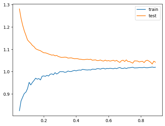
4 Feature engineering
- Linear with intercept: \(\hat y= \beta_0 + \boldsymbol{x}^T\boldsymbol{\beta}\).
Denoting the coordinates of \(x\) by \(x_1,\dots,x_P\), \[ \varphi:\mathbb{R}^P\to\mathbb{R}^{P+1}, \; \; \; \; \varphi(x) = (1,x_1,\dots,x_{P}). \] We add a column of \(1\)’s to \(\boldsymbol{X}\).
- Quadratic: \(\hat y= \boldsymbol{x}^T \boldsymbol{B}\boldsymbol{x}\) where \(\boldsymbol{B}\) is a \(P\times P\) matrix.
\[ \varphi:\mathbb{R}^P\to\mathbb{R}^{P(P+1)/2}, \; \; \; \; \varphi(x)=\{x_ix_j\}_{1\leq i \leq j \leq P}. \]
- Step function with cutoffs at known values, over a single feature.
Suppose we want \(\hat{y}\) to be constant when \(x\leq c\), and possibly another constant when \(x>c\). Then: \[ \varphi:\mathbb{R}\to\{0,1\}^2, \; \; \; \; \varphi(x)=(I(x\leq c), I(x>c)), \] where \(I(A)\) is in the indicator function assuming value \(1\) when the event \(A\) materializes and \(0\) otherwise.
We replace \(\boldsymbol{X}\) with a one-hot column for each step.
- Continuous piece-wise linear function, over a single feature.
Suppose we want \(\hat{y}\) to be affine (linear plus constant) when \(x\leq c\), and affine with possibly another slope when \(x>c\). We also want to constrain that the two affine functions have the same value when \(x=c\), so that \(\hat{y}\) as a function of \(x\) will be continuous. Then: \[ \varphi:\mathbb{R}\to\mathbb{R}^3, \; \; \; \; \varphi(x)=(1, xI(x\leq c), (x-c)I(x>c)). \]
- Is it possible to implement an infinite-dimensional feature mapping \(\varphi\)? That is, \(Q=\infty\).
It is impossible to compute \(\varphi(x)\) because it is inifinite, however there are ways of using infinite feature mappings in linear regression without having to directly compute \(\varphi(x)\). These are known as kernel methods.