| mage | habit | weight |
|---|---|---|
| 34 | nonsmoker | 6.96 |
| 31 | nonsmoker | 8.86 |
| 36 | nonsmoker | 7.51 |
| 31 | nonsmoker | 6.75 |
| 26 | nonsmoker | 6.69 |
Class introduction
Obligatory ML intro slide
Machine learning (ML) does amazing things these days.
Imagine some vacuous ML infographics here!
Beginning with these complex applications can obscure what we mean by “statistical prediction.” So let’s begin with a much simpler example.
What is machine learning?
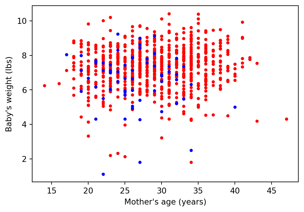
Every year, the US releases to the public a large data set containing information on births recorded in the country. This data set has been of interest to medical researchers who are studying the relation between habits and practices of expectant mothers and the birth of their children. This is a random sample of 1,000 cases from the data set released in 2014.
\(\vdots\)
Plot of the data
Three things we could do with this dataset
- Regress
weight ~ 1 + mage + habit. Ifhabitis statistically significant, warn mothers not to smoke. - Regress
weight ~ 1 + mage + habit. For a given mother, compute the expected baby weight. If it is low, recommend extra monitoring during the pregnancy. - Define a variable
low_weight = weight < 4. Run the logistic regressionlow_weight ~ 1 + mage + habit. For a given mother, compute the expected probability of low birth weight. If this probability is high, recommend extra monitoring during the preganancy.
Questions:
This class is called “Modern Statistical Prediction and Machine Learning”
- Which (if any) of these tasks is machine learning?
- Which (if any) of these tasks is prediction?
- Which (if any) are classification?
- Which (if any) is statistical?
- Which (if any) is modern?
Be prepared to justify your answers.
What is machine learning? What is prediction?
- Which (if any) of these tasks is machine learning?
- Which (if any) of these tasks is prediction?
Tasks 2 and 3 are prediction. One might also call them machine learning.
Task 1 is causal inference. We will not study causal inference, and I will strongly discourage ever interpreting our models causally.
Note: I depart from ISL on this point! They sometimes try to do “inference,” and carelessly (in my opinion).
What is machine learning? What is prediction?
In this course, “prediction” always take the following form:
- A fixed set of observed pairs \(\{(x_n, y_n)\}\), \(n=1,\ldots,N\).
- A (maybe hypothetical) set of \((x_*, \cdot)\) for which we want to guess or estimate the missing \(y_*\).
We use the observed data \(\{(x_n, y_n)\}\) to produce a function \(\hat{f}(\cdot)\) which we hope to use as a prediction
\[\hat{f}(x_*) =: \hat{y}_* \overset{\textrm{(hopefully)}}{\approx} y_* \].
Exercise: Give some examples where “prediction” in this sense might not refer to the future.
What is machine learning? What is prediction?
Here are some classical contemporary ML applications:
- Recognizing digits from pixelized images
- Generating human–like text
- Learning to play Go
- Finding cancer cells in an MRI image
- Automatically identifying the topics in a NYT article
- Finding genes with similar patterns of expression
Some of these don’t appear to be supervised learning problems.
This class will mostly focus on supervised learning, but with one unit on “unsupervised learning.”
What is classification?
Arguably, both tasks 2 and 3 are being used for prediction, since we are ultimately using our models to identify mothers who are at-risk for low birth weight babies.
However, in this class we will use these terms to describe the model, not the ultimate use.
Regression will mean a case where \(y_n\) takes values in \(\mathbb{R}^{}\).
Classification will mean a case where \(y_n\) takes values in an unordered, finite set (in this class, typically \(\{0, 1\}\)).
What is statistical?
None of these three procedures are inherently statistical. For example, you can use the OLS coefficients as descriptive statistics for this particular dataset, with no notion of random sampling.
But we all intuitively know that when we apply these results to future mothers, those mothers will be different somehow than the mothers we observed in this dataset.
How will they be different? As always, it depends how you use your model:
- The mothers may be observed at a different time (e.g. after these data were collected)
- The mothers may be from completely different populations (e.g. in another country)
- The mothers may be a different species (e.g. what happens if you expose a guinea pig to cigarette smoke)?
Quantifying these potential differences is hard.
What is statistical?
One way to imagine how the observed sample differs from the future population is to imagine that both are independent and identically distributed (IID) samples from the same population:
\[ (x_n, y_n) \overset{\mathrm{IID}}{\sim}p(x, y) \quad\textrm{and}\quad (x_*, y_*) \sim p(x, y) \quad\textrm{for the same }p. \]
An assumption of IID sampling is:
- Mathematically (fairly) tractable
- Usually false
- Maybe not a totally insane approximation to real–world variation
- Perhaps a plausible lower bound on the variation you really expect.
In this class, we will typically assume IID sampling, but keep an eye out for the consequences if it fails to hold.
What is statistical?
A lot of statistics classes begin by assuming there is a “true” parametric model for \(p(x, y)\) or for \(p(y\vert x)\).
For example, in an introductory linear regression class, you might see:
\[ \textrm{Assume } y_n = \boldsymbol{\beta}^\intercal\boldsymbol{x}_n + \varepsilon_n \quad\textrm{for}\quad\varepsilon_n \overset{\mathrm{IID}}{\sim}\mathcal{N}\left(0, \sigma^2\right). \]
In this class, we will never take such assumptions very seriously in real applications. The IID assumption is bad enough.
However, studying what would happen if such assumptions hold can provide some nice intuition that we might hope generalizes.
What is modern?
Before 2015, I believed a list of truths about machine learning:
- Good prediction balances bias and variance.
- You should not perfectly fit your training data as some in-sample errors can reduce out-of-sample error.
- High-capacity models don’t generalize.
- Optimizing to high precision harms generalization.
- Nonconvex optimization is hard in machine learning.
None of these are true. Or certainly, none are universal truths. … Given all of this evidence, why did we teach our undergrads a paradigm completely invalidated by empirical evidence? I don’t have an answer to that question.
What is modern?
Let’s not pretend otherwise: massive compute power, deep neural nets + stochastic gradient descent, and frictionless reproducibility have laid bare some major shortcomings in the theory you’ll be learning in this class.
So why learn this material?
- You still need to understand the simple settings we will study in this class to understand contemporary debates about how and why modern ML works
- Classical concepts still provide good practical guidance outside massive datasets + computing environments
- “Statistical ML” should arguably be the place where you learn the best mathematical principles we have
- This course provides vocabulary you need to participate in most scholarly discussion of machine learning
- Theory does not need to be perfect to be useful! (Take economic theory for example.)
What is modern?
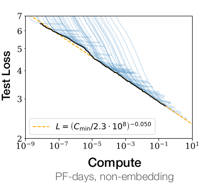
From Kaplan et al. (2020) Figure 1. The scaling of loss with compute is real, but slow!
A reliance on brute force computation puts the power of ML in the hands moneyed institutions.
Class organization
The class will focus on three types of problems:
- Supervised regression
- Supervised classification
- Unsupervised clustering
And on these interlocking key concepts:
- Loss minimization and generalization
- Ways to generate and control model complexity
- Computation
Each concept will be explored in the context of each problem. Hopefully you will see certain repetitive patterns emerge!
Bibliography
Kaplan, J., S. McCandlish, T. Henighan, T. Brown, B. Chess, R. Child, S. Gray, A. Radford, J. Wu, and D. Amodei. 2020. “Scaling Laws for Neural Language Models.” arXiv Preprint arXiv:2001.08361.