Linear regression in an ML setting

Goals

• Express ordinary least squares as loss minimization for IID data
• Discuss the advantages (but arbitrariness) of squared error
• Compare empirical and population losses
• Show consistency of OLS when we can use the LLN

Regression as loss minimization

Suppose we observe IID data,

\[ \mathcal{D}:= \left\{ (\boldsymbol{x}_n, y_n) \textrm{ for }n=1,\ldots,N \right\}. \]

Later, we expect to observe one (or more) values \(\boldsymbol{x}_\mathrm{new}\), but not the corresponding \(y_\mathrm{new}\). We’ll assume (tenuously!
unrealistically) that the pair \((\boldsymbol{x}_\mathrm{new}, y_\mathrm{new})\) come from the same distribution as the data, and are independent of the data.

To guess \(y_\mathrm{new}\), we want a function \(f(\boldsymbol{x}_\mathrm{new})\) for which we hope \(\hat{y}_\mathrm{new}:= f(\boldsymbol{x}_\mathrm{new})\) is “close” to \(y_\mathrm{new}\).

What does “close” mean? There are many choices for measuring a “distance” between \(\hat{y}_\mathrm{new}\) and \(y_\mathrm{new}\). Here are a few:

• \(|\hat{y}_\mathrm{new}- y_\mathrm{new}|\)
• \(|\hat{y}_\mathrm{new}- y_\mathrm{new}|^2\)
• \(|\hat{y}_\mathrm{new}- y_\mathrm{new}|^4\)
• \(\exp\left(|\hat{y}_\mathrm{new}- y_\mathrm{new}|\right)\)
• \(\mathrm{I}\left(|\hat{y}_\mathrm{new}- y_\mathrm{new}| > 1\right)\)
• \(\mathrm{I}\left(|\hat{y}_\mathrm{new}- y_\mathrm{new}| \ne 0\right)\)

Notation

In this course, \(\mathrm{I}\left(z\right)\) will always be the “indicator function” taking value \(0\) when \(z\) is false and \(1\) when \(z\) is true.

Whichever one we choose, we’ll define the “loss” of guessing \(\hat{y}\) when the true value was is \(y\) as \[ \mathscr{L}(\hat{y}, y) = \mathscr{L}(f(\boldsymbol{x}), y) \]

We want to find \(f(\cdot)\) so that \(\mathscr{L}(f(\boldsymbol{x}), y)\) is as small as possible. But the loss for a particular \(f\) may depend on \(\boldsymbol{x}_\mathrm{new}\), since different \(\boldsymbol{x}_\mathrm{new}\) are associated with different distributions of \(y_\mathrm{new}\). It follows that it doesn’t make sense to minimize the loss — instead we want to minimize the risk,

\[ \begin{aligned} \mathscr{L}(f) :=& \mathbb{E}_{\,}\left[\mathscr{L}(f(\boldsymbol{x}), y)\right] & \textrm{(Risk)}. \end{aligned} \]

Warning

Note the shorthand \(\mathscr{L}(f) := \mathbb{E}_{\,}\left[\mathscr{L}(f(\boldsymbol{x}), y)\right]\); loss as a function of a candidate function alone will be understood to be the expected loss of the candidate function evaluated at a new datapoint, that is, the risk. I think the double use of the notation \(\mathscr{L}(\cdot)\) is justified in order to avoid a profusion of symbols, but I apologize if it causes confusion.

A quick stroll through the internet suggests that “risk” and “loss” are somewhat inconsistently defined, so the main thing is to keep track of what you mean in a particular case.

So we would like to find

\[ f^{\star}(\cdot) := \underset{f}{\mathrm{argmin}}\, \mathscr{L}(f) = \underset{f}{\mathrm{argmin}}\, \mathbb{E}_{\,}\left[\mathscr{L}(f(\boldsymbol{x}), y)\right]. \]

Notation

The \(\underset{\,}{\mathrm{argmin}}\,\) operator finds the argument that minimizes a function, as opposed to the actual minimum, which is returned by \(\min{\,}\). For example

\[ \min{x}{(x - 3)^2 + 4} = 4 \quad\textrm{and}\quad \underset{x}{\mathrm{argmin}}\,{(x - 3)^2 + 4} = 3, \]

since the function \((x - 3)^2 + 4\) is minimized at the \(\underset{\,}{\mathrm{argmin}}\,\) value \(x= 3\), at which point it takes the \(\min{\,}\) value \(4\).

Notation

The notation \((\cdot)\) in \(f^{\star}(\cdot)\) emphasizes that the object \(f^{\star}\) is a function. In contrast, I will (try) to write \(f^{\star}(x)\) only for the function \(f^{\star}\) evaluate at a particular value \(x\).

The problem with this definition of \(f^{\star}\) is that we don’t actually know how to compute \(\mathscr{L}(f)\), since we don’t know the joint distribution of \(\boldsymbol{x},y\). In this class, we will extensively use and study the empirical loss,

\[ \hat{\mathscr{L}}(f) := \frac{1}{N} \sum_{n=1}^N\mathscr{L}(f(\boldsymbol{x}_n), y_n). \]

By the law of large numbers, for any particular \(f\), we might expect that \(\hat{\mathscr{L}}(f) \approx \mathscr{L}(f)\):

\[ \hat{\mathscr{L}}(f) \rightarrow \mathscr{L}(f) \quad\textrm{for a particular $f$, by the LLN}. \]

But that is not enough, since what we want is for

\[ \underset{f}{\mathrm{argmin}}\, \hat{\mathscr{L}}(f) \approx \underset{f}{\mathrm{argmin}}\, \mathscr{L}(f). \]

For example, what if \(\mathscr{L}(f') = \mathscr{L}(f)\), but, at a particular \(N\), \(\hat{\mathscr{L}}(f')\) is systematically lower than \(\hat{\mathscr{L}}(f)\)? This can happen when the function \(f'\) overfits the randomness in the dataset at hand.

One of the key themes of statistical machine learning, and of this class, is when and why \(\hat{\mathscr{L}}\) is an appropriate proxy for \(\mathscr{L}\).

Linear regression and least squares loss

For the next few weeks, we will focus on least squares loss \(\mathscr{L}(\hat{y}, y) = (\hat{y}- y)^2\). This loss does not always reflect what we really want, but it is extremely computationally and analytically tractable, and so widely used.

Given some \(\boldsymbol{x}_\mathrm{new}\), we want to find a best guess \(f(\boldsymbol{x}_\mathrm{new})\) for the value of \(y_\mathrm{new}\): specifically, we want to find the function that minimizes the “loss”

\[ f^{\star}(\cdot) := \underset{f}{\mathrm{argmin}}\, \mathbb{E}_{\,}\left[\mathscr{L}(y_\mathrm{new}, f(\boldsymbol{x}_\mathrm{new}))\right] = \underset{f}{\mathrm{argmin}}\, \mathbb{E}_{\,}\left[\left( y_\mathrm{new}- f(\boldsymbol{x}_\mathrm{new}) \right)^2\right]. \]

This is a functional optimization problem over an infinite dimensional space! You can solve this using some fancy math, but you can also prove directly that the best choice is

\[ f^{\star}(\boldsymbol{x}_\mathrm{new}) = \mathbb{E}_{\,}\left[y_\mathrm{new}| \boldsymbol{x}_\mathrm{new}\right]. \]

Suppose we consider any other function \(f(\cdot)\). The loss is larger, since

\[ \begin{aligned} \mathbb{E}_{\,}\left[\left( y_\mathrm{new}- f(\boldsymbol{x}_\mathrm{new}) \right)^2\right] ={}& \mathbb{E}_{\,}\left[ \mathbb{E}_{\,}\left[\left( y_\mathrm{new}- f(\boldsymbol{x}_\mathrm{new}) \right)^2 | \boldsymbol{x}_\mathrm{new}\right] \right] &\textrm{(Tower property)} \\={}& \mathbb{E}_{\,}\left[ \mathbb{E}_{\,}\left[\left( y_\mathrm{new}- f^{\star}(\boldsymbol{x}_\mathrm{new}) + f^{\star}(\boldsymbol{x}_\mathrm{new}) - f(\boldsymbol{x}_\mathrm{new}) \right)^2 | \boldsymbol{x}_\mathrm{new}\right] \right] &\textrm{(add and subtract)} \\={}& \mathbb{E}_{\,}\left[\left( y_\mathrm{new}- f^{\star}(\boldsymbol{x}_\mathrm{new}) \right)^2\right] + \\& \mathbb{E}_{\,}\left[\left( f^{\star}(\boldsymbol{x}_\mathrm{new}) - f(\boldsymbol{x}_\mathrm{new}) \right)^2\right] + \\& 2 \mathbb{E}_{\,}\left[ \mathbb{E}_{\,}\left[y_\mathrm{new}- f^{\star}(\boldsymbol{x}_\mathrm{new}) | \boldsymbol{x}_\mathrm{new}\right] \left( f^{\star}(\boldsymbol{x}_\mathrm{new}) - f(\boldsymbol{x}_\mathrm{new}) \right) \right] &\textrm{(expand the quadratic, use conditioning)} \\={}& \mathbb{E}_{\,}\left[\left( y_\mathrm{new}- f^{\star}(\boldsymbol{x}_\mathrm{new}) \right)^2\right] + \\& \mathbb{E}_{\,}\left[\left( f^{\star}(\boldsymbol{x}_\mathrm{new}) - f(\boldsymbol{x}_\mathrm{new}) \right)^2\right] + & \textrm{($\mathbb{E}_{\,}\left[y_\mathrm{new}- f^{\star}(\boldsymbol{x}_\mathrm{new}) | \boldsymbol{x}_\mathrm{new}\right]=0$ by definition)} \\\ge& \mathbb{E}_{\,}\left[\left( y_\mathrm{new}- f^{\star}(\boldsymbol{x}_\mathrm{new}) \right)^2\right]. & \textrm{(anything squared is greater than $0$)} \end{aligned} \]

Approximating the conditional expectation

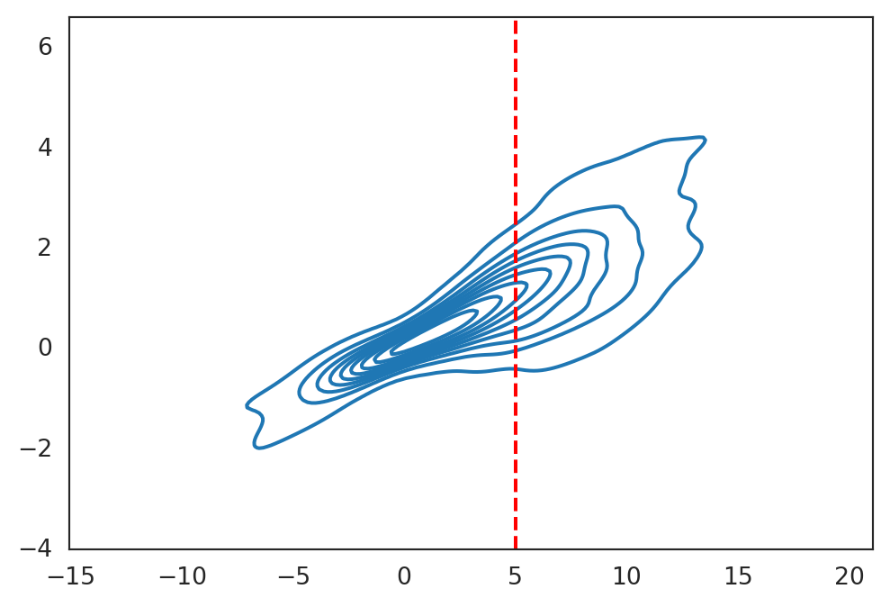
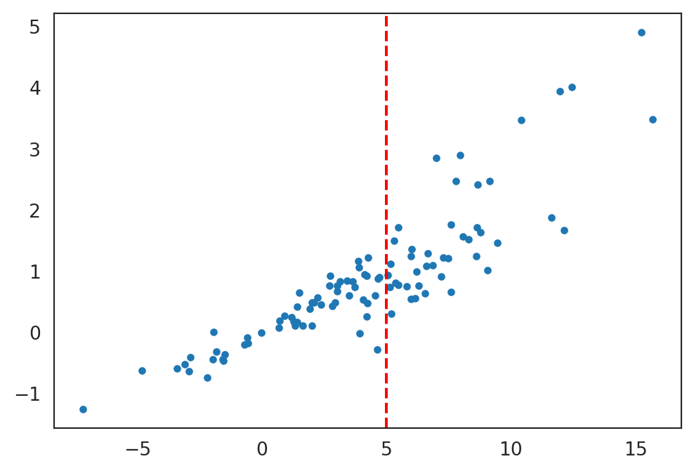
We now know that the optimal regression function is given by \(f^{\star}(\boldsymbol{x}) = \mathbb{E}_{\,}\left[y| \boldsymbol{x}\right]\). The problem is how to estimate it.

We have been imagining that we know the full joint distribution of \(\boldsymbol{x}\) and \(y\). In that case, we can read off the conditional distribution by “slicing” through a particular \(\boldsymbol{x}\):

However, in practice, we don’t actually observe the full joint distribution, we observe data points. How should we proceed?

Linear approximation

Typically, we don’t know the functional form of \(\mathbb{E}_{\,}\left[y| \boldsymbol{x}\right]\), because we don’t know the joint distribution of \(\boldsymbol{x}\) and \(y\). But suppose we approximate it with

\[ \mathbb{E}_{\,}\left[y| \boldsymbol{x}\right] \approx \boldsymbol{\beta}^\intercal\boldsymbol{x}. \]

Note that we are not assuming this is true — we do not expect that \(\mathbb{E}_{\,}\left[y| \boldsymbol{x}\right]\) is a linear function of \(\boldsymbol{x}\). Rather, we are finding the best approximation to the unknown \(\mathbb{E}_{\,}\left[y_\mathrm{new}| \boldsymbol{x}_\mathrm{new}\right]\) amongst the class of functions of the form \(\boldsymbol{\beta}^\intercal\boldsymbol{x}_\mathrm{new}\).

The linear assumption gives us a finite–dimensional class of candidate functions, which gives us a tractable optimization problem. Under this approximation, the problem becomes \[ \begin{aligned} \beta^{*}:={}& \underset{\beta}{\mathrm{argmin}}\, \mathbb{E}_{\,}\left[\left( y- \boldsymbol{\beta}^\intercal\boldsymbol{x}\right)^2\right] \\ ={}& \underset{\beta}{\mathrm{argmin}}\, \left(\mathbb{E}_{\,}\left[y^2\right] - 2 \boldsymbol{\beta}^\intercal\mathbb{E}_{\,}\left[y\boldsymbol{x}\right] + \boldsymbol{\beta}^\intercal\mathbb{E}_{\,}\left[\boldsymbol{x}\boldsymbol{x}^\intercal\right] \boldsymbol{\beta}\right). \end{aligned} \]

Differentiating with respect to \(\boldsymbol{\beta}\) and solving gives

\[ \boldsymbol{\beta}^{*}= \mathbb{E}_{\,}\left[\boldsymbol{x}\boldsymbol{x}^\intercal\right] ^{-1} \mathbb{E}_{\,}\left[\boldsymbol{x}y\right]. \]

Empirical approximation

Now, we cannot actually compute \(\beta^{*}\), since we still don’t know the joint distribution of \(\boldsymbol{x}\) and \(y\), and so cannot compute the preceding expectations. However, if we have a training set, we can approximate the expected loss:

\[ \hat{\boldsymbol{\beta}}:= \underset{\boldsymbol{\beta}}{\mathrm{argmin}}\, \frac{1}{N} \sum_{n=1}^N\left( y_n - \boldsymbol{\beta}^\intercal\boldsymbol{x}_n \right)^2 = \underset{\boldsymbol{\beta}}{\mathrm{argmin}}\, \hat{\mathscr{L}}(\boldsymbol{\beta}) \overset{?}{\approx} \underset{\boldsymbol{\beta}}{\mathrm{argmin}}\, \mathbb{E}_{\,}\left[\left( y- \boldsymbol{\beta}^\intercal\boldsymbol{x}\right)^2\right] = \underset{\boldsymbol{\beta}}{\mathrm{argmin}}\, \mathscr{L}(\boldsymbol{\beta}) = \boldsymbol{\beta}^{*}. \]

Recall that we can write the objective function for \(\hat{\boldsymbol{\beta}}\) in matrix notation as

\[ \hat{\boldsymbol{\beta}}:= \underset{\boldsymbol{\beta}}{\mathrm{argmin}}\, (\boldsymbol{Y}- \boldsymbol{X}\boldsymbol{\beta})^\intercal(\boldsymbol{Y}- \boldsymbol{X}\boldsymbol{\beta}) =: \underset{\boldsymbol{\beta}}{\mathrm{argmin}}\, \hat{\mathscr{L}}(\boldsymbol{\beta}), \]

Setting derivatives with respect to \(\boldsymbol{\beta}\) equal to zero gives

\[ \left. \frac{\partial \hat{\mathscr{L}}(\boldsymbol{\beta})}{\partial \boldsymbol{\beta}} \right|_{\hat{\boldsymbol{\beta}}} = 2 \boldsymbol{X}^\intercal\boldsymbol{Y}- 2 \boldsymbol{X}^\intercal\boldsymbol{X}\hat{\boldsymbol{\beta}}= \boldsymbol{0}. \]

When \(\boldsymbol{X}^\intercal\boldsymbol{X}\) is invertible (i.e., \(\boldsymbol{X}\) is full rank), then

\[ \hat{\boldsymbol{\beta}}= (\boldsymbol{X}^\intercal\boldsymbol{X})^{-1} \boldsymbol{X}^\intercal\boldsymbol{Y}= \left(\frac{1}{N} \boldsymbol{X}^\intercal\boldsymbol{X}\right)^{-1} \frac{1}{N} \boldsymbol{X}^\intercal\boldsymbol{Y}. \]

Consistency

If we can apply a LLN, then

\[ \frac{1}{N} \boldsymbol{X}^\intercal\boldsymbol{X}\rightarrow \mathbb{E}_{\,}\left[\boldsymbol{x}\boldsymbol{x}^\intercal\right] \quad\textrm{and}\quad \frac{1}{N} \boldsymbol{X}^\intercal\boldsymbol{Y}\rightarrow \mathbb{E}_{\,}\left[\boldsymbol{x}y\right], \]

and so (by the continuous mapping theorem if \(\mathbb{E}_{\,}\left[\boldsymbol{x}\boldsymbol{x}^\intercal\right]\) is invertible),

\[ \hat{\boldsymbol{\beta}}\rightarrow \boldsymbol{\beta}^{*}. \]

In other words, the OLS estimator is a consistent estimator of \(\boldsymbol{\beta}^{*}\) when we can apply the LLN and continuous mapping theorem to the quantities \(\boldsymbol{x}\boldsymbol{x}^\intercal\) and \(\boldsymbol{x}y\).

The preceding proof of the consistency of \(\hat{\boldsymbol{\beta}}\) used an explicit formula for \(\hat{\boldsymbol{\beta}}\). In this class, we will often discuss estimators for whom no explicit formula exists because we will find them via black–box optimization procedures. How can we reason in such cases?

Recall that we argued, for a particular \(f\), that a LLN should give

\[ \hat{\mathscr{L}}(f) \rightarrow \mathscr{L}(f). \]

For the OLS case, this expression is the same as

\[ \begin{aligned} \hat{\mathscr{L}}(\boldsymbol{\beta}) ={}& \frac{1}{N} \sum_{n=1}^N(\boldsymbol{x}_n^\intercal\boldsymbol{\beta}- y_n)^2 \\={}& \frac{1}{N} \sum_{n=1}^N\boldsymbol{\beta}^\intercal\boldsymbol{x}_n \boldsymbol{x}_n^\intercal\boldsymbol{\beta}- 2\frac{1}{N} \sum_{n=1}^N\boldsymbol{\beta}^\intercal\boldsymbol{x}_n y_n + \frac{1}{N} \sum_{n=1}^Ny_n^2 \\={}& \boldsymbol{\beta}^\intercal\left(\frac{1}{N} \sum_{n=1}^N\boldsymbol{x}_n \boldsymbol{x}_n^\intercal\right) \boldsymbol{\beta}- 2 \boldsymbol{\beta}^\intercal\left(\frac{1}{N} \sum_{n=1}^N\boldsymbol{x}_n y_n \right) + \frac{1}{N} \sum_{n=1}^Ny_n^2 \\\rightarrow{}& \boldsymbol{\beta}^\intercal\mathbb{E}_{\,}\left[\boldsymbol{x}\boldsymbol{x}^\intercal\right] \boldsymbol{\beta}- 2 \boldsymbol{\beta}^\intercal\mathbb{E}_{\,}\left[ \boldsymbol{x}y\right] + \mathbb{E}_{\,}\left[y_n^2\right] \\={}& \mathbb{E}_{\,}\left[(\boldsymbol{x}^\intercal\boldsymbol{\beta}- y)^2 \right] \\={}& \mathscr{L}(\boldsymbol{\beta}). \end{aligned} \]

Unfortunately, this does not translate directly into \(\hat{\boldsymbol{\beta}}\rightarrow \boldsymbol{\beta}^{*}\), since the preceding limit holds only for a fixed \(\boldsymbol{\beta}\). Different \(\boldsymbol{\beta}\) will lead to convergence at different rates, so in theory it may be the case that \(\underset{\boldsymbol{\beta}}{\mathrm{argmin}}\, \hat{\mathscr{L}}(\boldsymbol{\beta})\) does not converge to \(\underset{\boldsymbol{\beta}}{\mathrm{argmin}}\, \mathscr{L}(\boldsymbol{\beta})\).

Further, in practice, we really don’t care about learning the function \(\boldsymbol{\beta}^{*}\), rather we want to achieve the optimal loss. That is, we are interested in the ``regret’’

\[ \textrm{Regret}(\hat{\boldsymbol{\beta}}) := \mathscr{L}(\hat{\boldsymbol{\beta}}) - \mathscr{L}(\boldsymbol{\beta}^{*}) \ge 0. \]

That is, by using \(\hat{\boldsymbol{\beta}}\) instead of the optimal \(\boldsymbol{\beta}^{*}\), how much worse is our ``true’’ loss? Note that this quantity must be positive since you cannot do better than \(\boldsymbol{\beta}^{*}\), but we would like to show that \(\mathscr{L}(\hat{\boldsymbol{\beta}}) - \mathscr{L}(\boldsymbol{\beta}^{*}) \rightarrow 0\). But we really don’t know much about \(\mathscr{L}(\hat{\boldsymbol{\beta}})\), so we need to express the regret in terms of quantities we understand.

Uniform laws

A useful decomposition is as follows:

\[ \begin{aligned} 0 \le \mathscr{L}(\hat{\boldsymbol{\beta}}) - \mathscr{L}(\boldsymbol{\beta}^{*}) ={}& \mathscr{L}(\hat{\boldsymbol{\beta}}) - \hat{\mathscr{L}}(\hat{\boldsymbol{\beta}}) & \textrm{Difficult term!}\\ & + \hat{\mathscr{L}}(\hat{\boldsymbol{\beta}}) - \hat{\mathscr{L}}(\boldsymbol{\beta}^{*}) & \textrm{Negative term} \\ & + \hat{\mathscr{L}}(\boldsymbol{\beta}^{*}) - \mathscr{L}(\boldsymbol{\beta}^{*}) & \textrm{LLN term} \end{aligned} \]

We wish to bound the preceding equation by a quantity that goes to zero; if we do, then \(\mathscr{L}(\hat{\boldsymbol{\beta}}) - \mathscr{L}(\boldsymbol{\beta}^{*}) \rightarrow 0\).

The second term is negative, since \(\hat{\boldsymbol{\beta}}\) minimizes \(\hat{\mathscr{L}}\), and so \(\hat{\mathscr{L}}(\hat{\boldsymbol{\beta}}) \le \hat{\mathscr{L}}(\boldsymbol{\beta})\) for any \(\boldsymbol{\beta}\), and for \(\boldsymbol{\beta}^{*}\) in particular. So it is bounded above by zero, and we don’t need to consider it any further.

The third term goes to zero by the LLN, since \(\boldsymbol{\beta}^{*}\) is fixed.

However, the first “difficult” term does not necessarily go to zero by the LLN, since \(\hat{\boldsymbol{\beta}}\) is random and correlated with \(\hat{\mathscr{L}}\). Specifically, in

\[ \hat{\mathscr{L}}(\hat{\boldsymbol{\beta}}) = \frac{1}{N} \sum_{n=1}^N(y_n - \boldsymbol{x}_n^\intercal\hat{\boldsymbol{\beta}})^2, \]

the entries \((y_n - \boldsymbol{x}_n^\intercal\hat{\boldsymbol{\beta}})^2\) are not IID, since \(\hat{\boldsymbol{\beta}}\) depends on all the entries.

One standard way of dealing with terms of the form \(\hat{\mathscr{L}}(\hat{\boldsymbol{\beta}}) - \mathscr{L}(\hat{\boldsymbol{\beta}})\) is uniform laws of large numbers or ULLNs. For some compact set \(K\), a ULLN for this setting would state that a LLN holds uniformly over \(K\).

\[ \begin{aligned} \textrm{For a fixed }\boldsymbol{\beta}\textrm{, } \left|\hat{\mathscr{L}}(\boldsymbol{\beta}) - \mathscr{L}(\boldsymbol{\beta})\right| \rightarrow {}& 0 & \textrm{(LLN)} \\ \sup_{\beta \in K} \left|\hat{\mathscr{L}}(\boldsymbol{\beta}) - \mathscr{L}(\boldsymbol{\beta})\right| \rightarrow {}& 0 & \textrm{(ULLN)}. \end{aligned} \]

If a ULLN holds, and we believe that \(\hat{\boldsymbol{\beta}}\in K\), then

\[ \left|\mathscr{L}(\hat{\boldsymbol{\beta}}) - \hat{\mathscr{L}}(\hat{\boldsymbol{\beta}})\right| \le \sup_{\boldsymbol{\beta}\in K} \left|\mathscr{L}(\boldsymbol{\beta}) - \hat{\mathscr{L}}(\boldsymbol{\beta})\right| \rightarrow 0, \]

and so

\[ \mathscr{L}(\hat{\boldsymbol{\beta}}) - \mathscr{L}(\boldsymbol{\beta}^{*}) \rightarrow 0. \]

It turns out that it is easy to state condtiions under which a ULLN holds for linear regression. In general, we get a ULLN by limiting the complexity of our function class, as we will see later in the class.